A tour of Quantitative Text Analysis

The workshop started with a few basics: While QTA can be efficient and cheap, it always fails to rely on a correct model of language. It does not free us from reading texts, and validation is key. We learned about the basic distinction between classification (organizing text into categories) and scaling (estimation positions of actors), and its supervised (where hand-coded or other external data is available) and unsupervised (without such data) variants.

(Pre-)processing text

We relied on the R package quanteda developed by Ken Benoit and collaborators, which takes QTA by storm, at least for those working in R. Together with the readtext package, it easily allows to get your text data into R, create a so-called “corpus” of texts with the actual content as well as meta-information, and perform various tasks of corpus and text processing (subsetting a corpus, creating a document-feature matrix (dfm), stopword removal) as well as analysis (scaling, classification). A large and increasing number of extras is also available, such as ways to assess text similarity (function textsta_simil()) and lexical diversity (textstat_lexdiv()). Some of these features are demonstrated in an example below. Also see this overview by quanteda for a full list of functions and the preText package for advise on evaluating pre-processing specifications.

A small coalition corpus

For a few examples from the workshop, consider a small set of three documents: The coalition agreement between the CDU/CSU and the SPD as well as the respective election manifestos from the 2017 Bundestag election. The corpus is created by:

library(readtext)
library(quanteda)
text <- readtext(paste0(wd, "coalition/*.txt"),
                 docvarsfrom = "filenames",
                 docvarnames = "Party")
text$text <- gsub("\n", " ", text$text)
coalitioncorpus <- corpus(text, docid_field = "doc_id")
coalitioncorpus$metadata$source <- "[directory] on [system] by [user]"
summary(coalitioncorpus)

## Corpus consisting of 3 documents:
## 
##           Text Types Tokens Sentences     Party
##     cducsu.txt  4738  26004      1288    cducsu
##  coalition.txt 11660  93214      3763 coalition
##        spd.txt  7650  50298      2402       spd
## 
## Source: [directory] on [system] by [user]
## Created: Wed Nov 11 15:06:41 2020
## Notes:

The code relies on the two packages, readtext and quanteda, to create a data frame with the text files, using their names for a document-level variable called “Party”. The gsub() command removes whitespace, and corpus() turns the data frame into a corpus, which is a special case of a data frame containing texts, some meta-information and document-level variables, all optimized to perform a variety of quantitative text analysis operations using quanteda.

Further document-level variables are added via:

docvars(coalitioncorpus, "Year") <- 2017
docvars(coalitioncorpus, "Party_regex") <- 
  sub("[\\.].*", "", names(texts(coalitioncorpus)))
docvars(coalitioncorpus)

##                   Party Year Party_regex
## cducsu.txt       cducsu 2017      cducsu
## coalition.txt coalition 2017   coalition
## spd.txt             spd 2017         spd

Note that this uses a regular expression (regex) to alternatively retrieve the party names from the filenames after creating the corpus. For specific analyses, we want to know the distribution of words across documents and create a document-feature matrix (dfm):

dfm_coal <- dfm(
  coalitioncorpus,
  remove = c(stopwords("german"),
             "dass",
             "sowie",
             "insbesondere"),
  remove_punct = TRUE,
  stem = FALSE
)
dfm_coal[, 1:8]

## Document-feature matrix of: 3 documents, 8 features (16.7% sparse).
## 3 x 8 sparse Matrix of class "dfm"
##                features
## docs            gutes land zeit deutschland liebens lebenswertes gut
##   cducsu.txt        6   48   11         147       1            1  16
##   coalition.txt     1   39   14         195       0            0  13
##   spd.txt           6   44   33          97       0            0  17
##                features
## docs            wohnen
##   cducsu.txt         1
##   coalition.txt     10
##   spd.txt            6

Creating a dfm induces a bag-of-words assumption. This means that the order in which words appear is ignored. A dfm is a means of information reduction and the most efficient way of storing text as data, but allows only analyses under this assumption. We quickly glance at the similarity (function textstat_simil()) and lexical diversity (function textstat_lexdiv()) of texts:

simil <- textstat_simil(dfm_coal,
                        margin = "documents",
                        method = "correlation")
simil 

## textstat_simil object; method = "correlation"
##               cducsu.txt coalition.txt spd.txt
## cducsu.txt         1.000         0.968   0.975
## coalition.txt      0.968         1.000   0.986
## spd.txt            0.975         0.986   1.000

textstat_lexdiv(dfm_coal)[, 1:2]

##        document       TTR
## 1    cducsu.txt 0.3302084
## 2 coalition.txt 0.2487993
## 3       spd.txt 0.2802713

From this, we learn that the SPD manifesto has more similarity to the coalition agreement than that of the CDU/CSU, a notion which somewhat resembles the assessment of the 2017 German coalition. Also, the lexical diversity of the manifestos, measured in terms of types (different words) per token (total words), appears to be higher than the coalition agreement, especially for the CDU/CSU.

Sentiment analysis using a dictionary

For sentiment analyis, existing dictionaries are available. It is important to note that these do not necessarily fit the research question at hand. In this example, the German “LIWC” (linguistic inquiry and word count) dictionary is used, but alternatives exist, such as “Lexicoder” for political text. LIWC features the categories “anger”, “posemo” (positive emotion) and “religion”. After obtaining the dictionary and applying it while creating a dfm from the corpus, the share of the texts in the respective categories is displayed. The results indicate that the coalition agreement features less positive emotions as compared to the manifestos and that the SPD manifesto is the most “angry” text, while the CDU/CSU speaks most about religion.

# Create dictionary
liwcdict <- dictionary(file = paste0(wd, "German_LIWC2001_Dictionary.dic"),
                       format = "LIWC")

# Create dfm
liwcdfm <- dfm(
  coalitioncorpus,
  remove = c(stopwords("german")),
  remove_punct = TRUE,
  stem = FALSE,
  dictionary = liwcdict
)

# Subset and calculate percentage
liwcsub <-
  dfm_select(liwcdfm,
             pattern = c("Anger", "Posemo", "Relig"),
             selection = "keep")

liwcsub <- convert(liwcsub, to = "data.frame")
liwcsub$sum <- apply(dfm_coal, FUN = sum, 1)
liwcparties <- data.frame(
  docs = liwcsub$document,
  ShareAnger = liwcsub$Anger / liwcsub$sum,
  SharePosemo = liwcsub$Posemo / liwcsub$sum,
  ShareRelig = liwcsub$Relig / liwcsub$sum
)

liwcparties 

##            docs  ShareAnger SharePosemo  ShareRelig
## 1    cducsu.txt 0.004314995  0.06414959 0.005609493
## 2 coalition.txt 0.004666188  0.05050462 0.004074997
## 3       spd.txt 0.005550042  0.05697063 0.003454993

LDA topic modelling

LDA stands for Latent Dirichlet allocation. In a nutshell, the method represents texts as a mixture of topics, and simultaneously topics as mixtures of words. Fixing the number of topics to \(k = 5\), and using the topicmodels package, the command lda() delivers posterior probabilities of the topics for each document.

library(topicmodels)

# Preparation
dfm_coal <-
  dfm(
    coalitioncorpus,
    remove = c(
      stopwords("german"),
      "dass",
      "sowie",
      "insbesondere",
      "b",
      "z",
      "a",
      "u"
    ),
    remove_punct = TRUE,
    remove_numbers = TRUE,
    stem = FALSE
  )

dfm_coal <- dfm_wordstem(dfm_coal, language = "german")

# Define parameters
burnin <- 1000
iter <- 500
keep <- 50
seed <- 2010
ntopics <- 5

# Run LDA with 5 topics
ldaOut <- LDA(
  dfm_coal,
  k = ntopics,
  method = "Gibbs",
  control = list(
    burnin = burnin,
    iter = iter,
    keep = keep,
    seed = seed,
    verbose = FALSE
  )
)
# Posterior probabilities of the topics for each document
k <- posterior(ldaOut)

Interpretation is the difficult part. Each document can be expressed as a mixture of topics, and notwithstanding the precise meaning of the topics, we learn that all texts share content referring to topic 1, while the CDU/CSU manifesto also features topic 2 and the SPD manifesto topic 3 to some extent.

k$topics

##                       1          2          3          4          5
## cducsu.txt    0.5815482 0.02729874 0.36122496 0.01144536 0.01848272
## coalition.txt 0.6950774 0.03700023 0.06163624 0.10570834 0.10057777
## spd.txt       0.6755292 0.17646590 0.11404313 0.01837605 0.01558576

Wordfish Scaling

Wordfish scaling derives latent positions from texts based on a bag-of-words assumption. Here is an example relying on a set of Swiss manifestos, using only the sections on immigration. In preparation, a dfm is created while removing stopwords, stemming the remaining words and removing punctuation.

manifestos <- readtext(paste0(wd, "manifestos/*.txt"))
manifestocorpus <- corpus(manifestos)
dfm_manifesto <-
  dfm(
    manifestocorpus,
    remove = c(
      "gruen*",
      "sp",
      "sozialdemokrat*",
      "cvp",
      "fdp",
      "svp",
      "fuer",
      "dass",
      "koennen",
      "koennte",
      "ueber",
      "waehrend",
      "wuerde",
      "wuerden",
      "schweiz*",
      "partei*",
      stopwords("german")
    ),
    valuetype = "glob",
    stem = FALSE,
    remove_punct = TRUE
  )
dfm_manifesto <- dfm_wordstem(dfm_manifesto, language = "german")

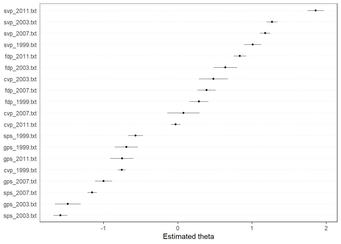
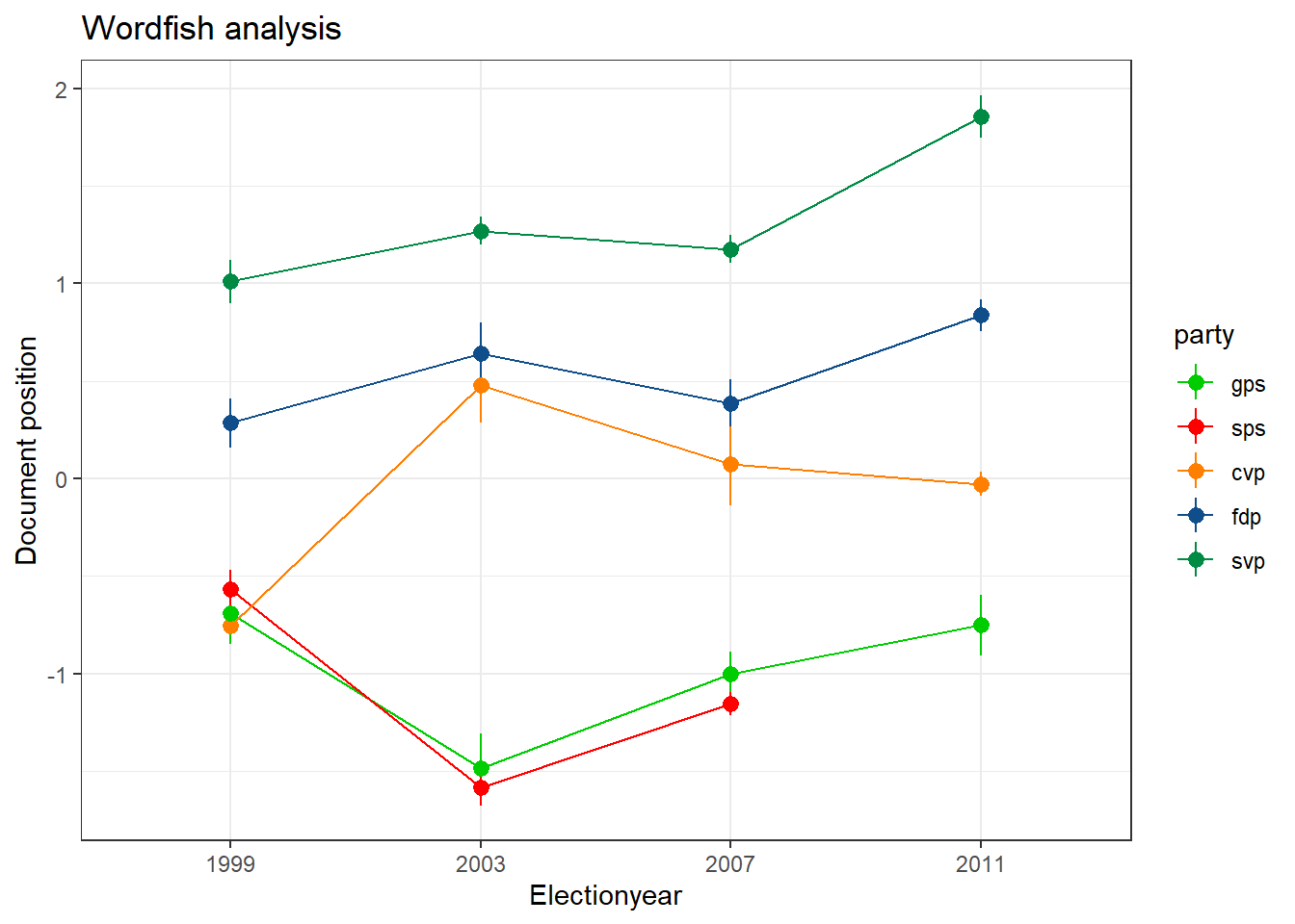
The function textmodel_wordfish() computes the Wordfish model, originally decribed in an AJPS article by Slapin and Proksch in 2009. It assumes that the distribution of words across texts follows a Poisson distribution, and can be modeled by document and word fixed effects as well as word-specific weights and document positions. The model is a variant of unsupervised scaling, only requiring the relative location of two texts on the latent dimension. Here, a text of the Swiss People’s Party (SVP) is assumed to be right to that of the Social Democratic Party of Switzerland (SPS). The results make some sense, with the other manifestos aligning as expected on what could be interpreted as a anti-immigration dimension.

wf <- textmodel_wordfish(dfm_manifesto,
                         dir = c(13, 19),
                         dispersion = "poisson")
textplot_scale1d(wf)

Or, with some improvements to the plot:

library(ggplot2)

# Save document scores and confidence intervals in data frame
wfdata <- as.data.frame(predict(wf, interval = "confidence"))

# Add document variables
wfdata$docs <- rownames(wfdata)
wfdata$electionyear <- substr(wfdata$docs, 5, 8)
wfdata$party <- as.factor(substr(wfdata$docs, 1, 3))
wfdata$party <-
  factor(wfdata$party, levels = c("gps", "sps", "cvp", "fdp", "svp"))

ggplot(wfdata) +
  geom_pointrange(
    aes(
      x = electionyear,
      y = fit.fit,
      ymin = fit.lwr,
      ymax = fit.upr,
      group = party,
      color = party
    ),
    size = 0.5
  ) +
  geom_line(aes(
    x = electionyear,
    y = fit.fit,
    group = party,
    color = party
  )) +
  theme_bw() +
  labs(title = "Wordfish analysis",
       y = "Document position",
       x = "Electionyear") +
  scale_color_manual(values = c("green3",
                                "red1",
                                "darkorange1",
                                "dodgerblue4",
                                "springgreen4"))

Further readings

• An introductory article to QTA in R, especially relying on quanteda: Welbers, Kasper, Wouter Van Atteveldt and Kenneth Benoit (2017): Text Analysis in R, Communication Methods and Measures 11(4): 245-65.
• An application of the methods by the workshop host and co-authors: Schwarz, Daniel, Denise Traber and Kenneth Benoit (2017): Estimating Intra-Party Preferences: Comparing Speeches to Votes. Political Science Research and Methods 5(2): 379-396.

About the presenter

Denise Traber is a Senior Research Fellow at the University of Lucerne, Switzerland, where she heads an Ambizione research grant project on “The divided people: polarization of political attitudes in Europe” funded by the Swiss National Science Foundation. She has a strong interest in quantitative text analysis, co-organizes the “Zurich Summer School for Women in Political Methodology” and has published the article “Estimating Intra-Party Preferences: Comparing Speeches to Votes” in Political Science Research and Methods in 2017, jointly with Daniel Schwarz and Ken Benoit.