LaTeX and Overleaf
LaTeX is a high quality typesetting system that that facilitates the production of well-formatted document. It has become highly popular in academic settings as an alternative to common typewriting systems (e.g., Word). This Methods Bites Tutorial by our team member Cosima Meyer and Dennis Hammerschmidt walks you through your first steps in LaTeX (using Overleaf) and provides you with a hands-on guide for writing scientific papers using an easily accessible template. It is based on the workshop Introduction to LaTeX and Overleaf at the MZES Social Science Data Lab in November 2019. The slides can be accessed on our GitHub.
This blog post includes:
- What is LaTeX and Overleaf
- First Steps in LaTeX
- LaTeX Template: A Hands-on Guide
- Further Readings (and Help)
- About the Presenters
What is LaTeX and Overleaf?
LaTeX
LaTeX was originally developed by Leslie Lamport in the 1980s as a user-friendly version of TeX. This is also how LaTeX came to its name: Lamport TeX. It is a high quality typesetting system with minimal effort that produces exactly the same results across all machines. It creates good looking text documents and is mostly used for technical reports and scientific articles. However, with LaTeX, you can also write books, generate presentations, posters, a professional looking CV/résumé, and much more. LaTeX offers many easy ways for customization, which allows you to adapt LaTeX to your personal needs and preferences. By default, however, LaTeX already tries to format a document in a nice looking way. Its vivid online community offers help in solving common challenges and initial difficulties can easily be overcome. This blogpost aims right at this: Introducing you to your first steps in LaTeX and providing you with a ready-to-use template for your scientific writing.
The main difference between LaTeX and a (probably more common) text processing system such as Word is that Word follows the logic of “what you see is what you get” (WYSIWYG). This means that you directly format the appearance of your text and document in Word and see the output instantly. In other words, selecting a word and hitting BOLD transforms the text you see in your document to bold right away. LaTeX, however, follows the idea of “what you see is what you mean” (WYSIWYM). This means that you enter a plain text and tell LaTeX with specific commands and functions the formatting you want. Instead of seeing the formatted output right away, as you do in Word, you only see the formatted output once LaTeX compiled your final document. By default, Overleaf produces PDF documents using the pdfLaTeX compiler.
Every LaTeX document consists of two parts: The preamble and the body. The preamble allows you to define all format requirements such as paper size or text width that are used throughout the entire document. Here, you can also load additional packages and define your preferred citation style. Basically, the preamble is used to define the general outline of what your document will look like but neither produces any written output nor appears in your final document. This means that, even if you write some plain text (e.g., your introduction section) in the preamble, LaTeX will not include it in the output of your final document.
The body, by contrast, is where you enter your main text that you also want to appear in your final document. You can easily spot this part as it is always encapsulated between \begin{document} and \end{document}. This means that everything between \begin{document} and \end{document} is visible in your final document whereas everything outside of this environment is not. If you, for example, write something after \end{document}, it will also not appear in your final PDF document.
However, in the spirit of WYSIWYM, basic (text) formatting can still be done in the body. We will introduce you to this in the following section. As you will see, while the body of your LaTeX file is dedicated for your plain text, specific commands allow you to still format your plain text individually. This is either done by wrapping an environment around it by defining a \begin{...} and \end{...} – similar to how you define the body of your document – or by applying a command directly to (a part of) the text that you want to format (e.g., \centering{Some text that should be centered.}).
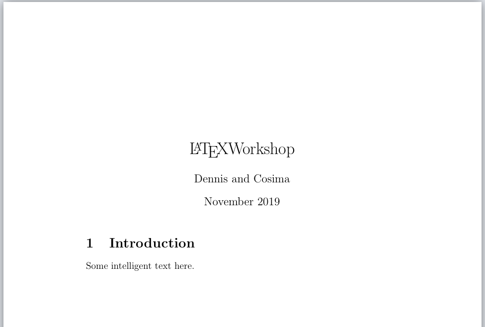
The following figures show you a simple example of how a LaTeX document is generally structured.
- Preamble: Here you define all the necessary settings (e.g., font, line spacing, load packages).
\documentclass[a4paper, 12 pt]{article}
\usepackage[utf8]{inputenc}

\author{Dennis and Cosima}
\title{\LaTeX Workshop}
\date{November 2019}- Body: Here you type your plain text. It is wrapped around the
documentenvironment with\begin{document}and\end{document}.
\begin{document}
\maketitle

\section{Introduction}
Some intelligent text here.
\end{document}
Bringing both parts together and compiling it to a PDF document, you will get the following:
Overleaf
There are two primary ways for using LaTeX. The first one is installing and running LaTeX on your local machine. The upside of this is that you have all your files readily available when you need them, even offline, and can compile your document on the go. The downside is that, if you refer to other files in your body, you need to keep track of the folder structure and need to know where all your files are stored in order to ensure smooth compiling. Additionally, you may be required to download and install packages manually (e.g., from the Comprehensive TeX Archive Network (CTAN)) on your machine before running them. This may become tricky when using some citation packages.
The second approach, and the one that we will focus on throughout this blogpost, is to use a cloud-based browser version of LaTeX. We will focus on one of the most popular web-based LaTeX editors: Overleaf. The upside of using this online editor is that Overleaf lets you store all necessary files in the cloud and thus allows you to access your files from every machine wherever you are – just in the spirit of LaTeX. This means that it also ensures that you have all files nicely stored in the necessary working directory. Moreover, Overleaf allows real-time collaboration with other users, has a smooth integration with popular citation systems and offers a wide range of templates. The basic version of Overleaf is free but can be updated with a subscription plan to collaborate with more colleagues or to add additional features. The downside is that, in order to compile your document via Overleaf, an internet connection is required. However, downloading all source code and files and using a local LaTeX compiler on your machine is still possible.
Due to its easy use and possibility to share our template – which we will introduce below – we provide the following introduction of LaTeX as shown in Overleaf. It is important to note that you can still reproduce all steps using a local LaTeX editor on your computer and can also download the template as a .zip file.
First Steps in LaTeX
Basics in LaTeX
To follow the steps below, you either need to create an account on Overleaf or get LaTeX as a desktop version as mentioned above.
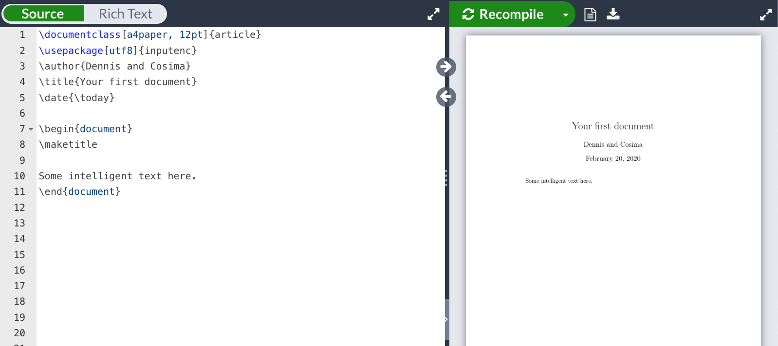
We open an empty document and start with the very minimal requirements you need for a LaTeX document to compile: A preamble and some text between \begin{document} and \end{document}. For now, our preamble includes just information on the documentclass (we use article here).
While this is a very basic document, you may want to become a bit more creative. The preamble usually includes much more – such as specific font sizes, your name, the title of the document, the date, and also additional packages that you may need for your document. Here is a short example. Adding to our previous document, we now also specify a page format (a4paper) and the font size (12pt). These settings are now set as the default for the entire document; but, as you will see below, modifications such as changing the font size is still possible for selected parts of your text.
Paper setting
\documentclass[a4paper, 12 pt]{article}

\begin{document}
Some intelligent text here.
\end{document}
In a next step, we load our very first package: inputenc. This package comes in handy to display the standard utf 8 encoding. Including packages is always done using \usepackage{...} in the preamble.
One important aspect of LaTeX that holds across both packages and general commands in the body is the use of squared brackets between the command name, here \usepackage and the curly brackets. As seen below, \usepackage[utf8]{inputenc} loads the inputenc package but has a further specification for the package, namely that it should be able to deal with utf8 characters. In LaTeX, if you want to add further specifications to a command, this is almost always done using squared brackets between the command name and the input in the curly brackets. We will encounter several of these specifications below.
Load
inputenc package
\documentclass[a4paper, 12 pt]{article}
\usepackage[utf8]{inputenc}

\begin{document}
Some intelligent text here.
\end{document}
Next, we add the authors’ names (\author{...}), the title of the document (\title{...}) and a date (\date{...}). You can include an automatic date with \today – this will always show the current date.
All this information is defined in the preamble. To refer to it and include it in our body, we need to tell LaTeX explicitly to do so and write \maketitle in the body.
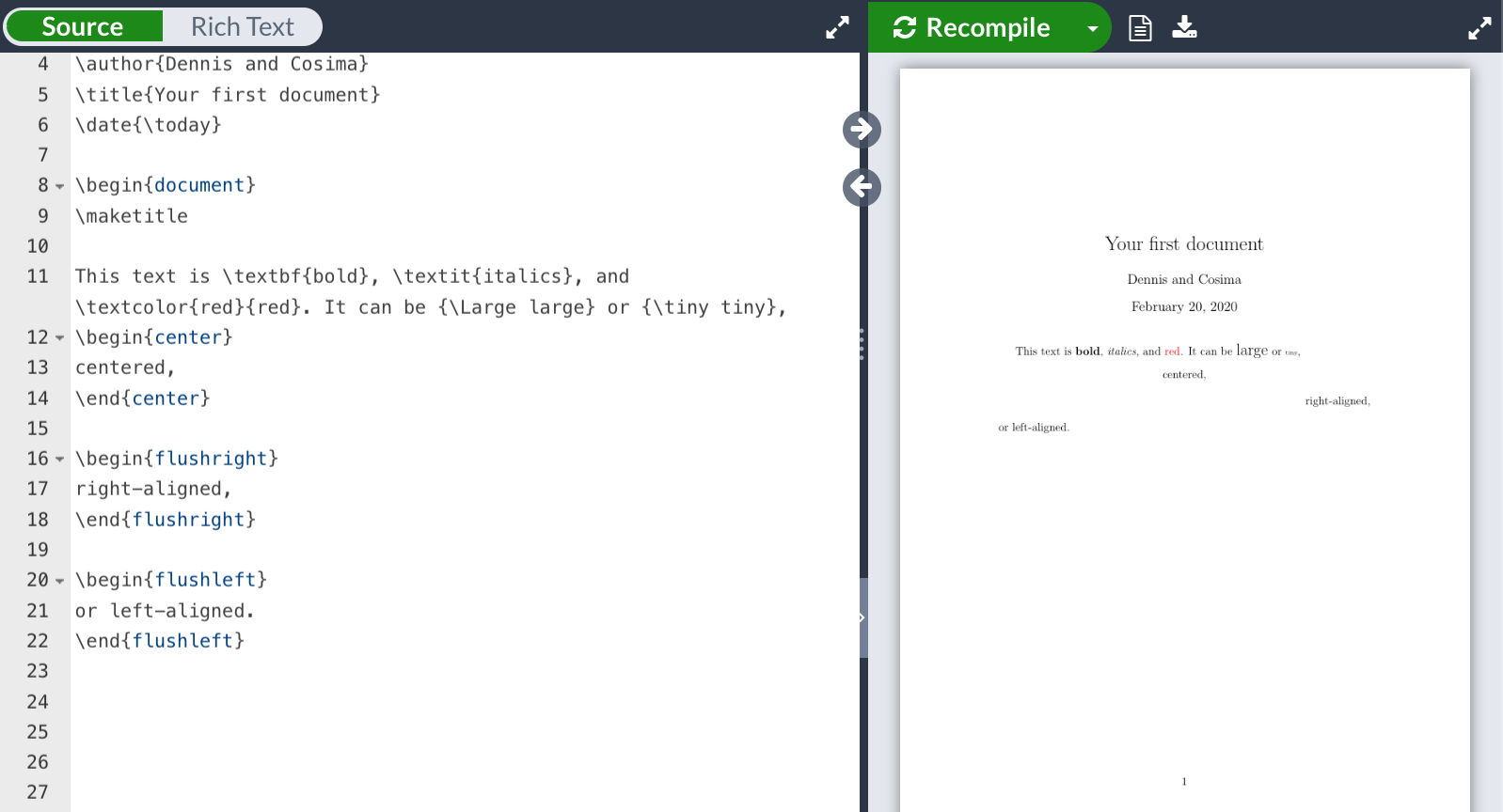
To re-emphasize, you pre-define everything that is necessary for the appearance of your document in the preamble and leave the body to your plain text. If you want to perform some (individual) basic formatting in the body, LaTeX allows you to do this by using commands. Common text formatting needs such as bold or cursive (italic) font can simply be evoked using \textbf{...} or \textit{...}, respectively, around the text snippet that should be formatted. Below is a quick list for reference of further, common text formats. More advanced formatting options usually follow the same principle and can easily be identified using a quick online search.
| bold |
\textbf{...}
|
| cursive (italic) |
\textit{...}
|
| colored text |
\textcolor{color}{...} (requires the package xcolor)
|
| font size |
\Huge, \huge, \LARGE, \Large, \large, \normalsize, \small, \footnotesize, \scriptsize, \tiny
|
| centered text |
\begin{center} ... \end{center}
|
| right aligned text |
\begin{flushright} ... \end{flushright}
|
| left aligned text |
\begin{flushleft} ... \end{flushleft}
|
| justified text | default |
Figure: Text formatting in action
Besides text formatting, other basic text features that can be edited in the body are sections or subsections as well as footnotes. Both follow the same logic as above. To define a section or heading, wrap \section{...} or \subsection{...} around your section title(s). The same holds for footnotes. The text within \footnote{...} is set as a footnote. LaTeX also counts automatically and adjusts the numbering of your footnotes if you have added or removed a footnote from your text.
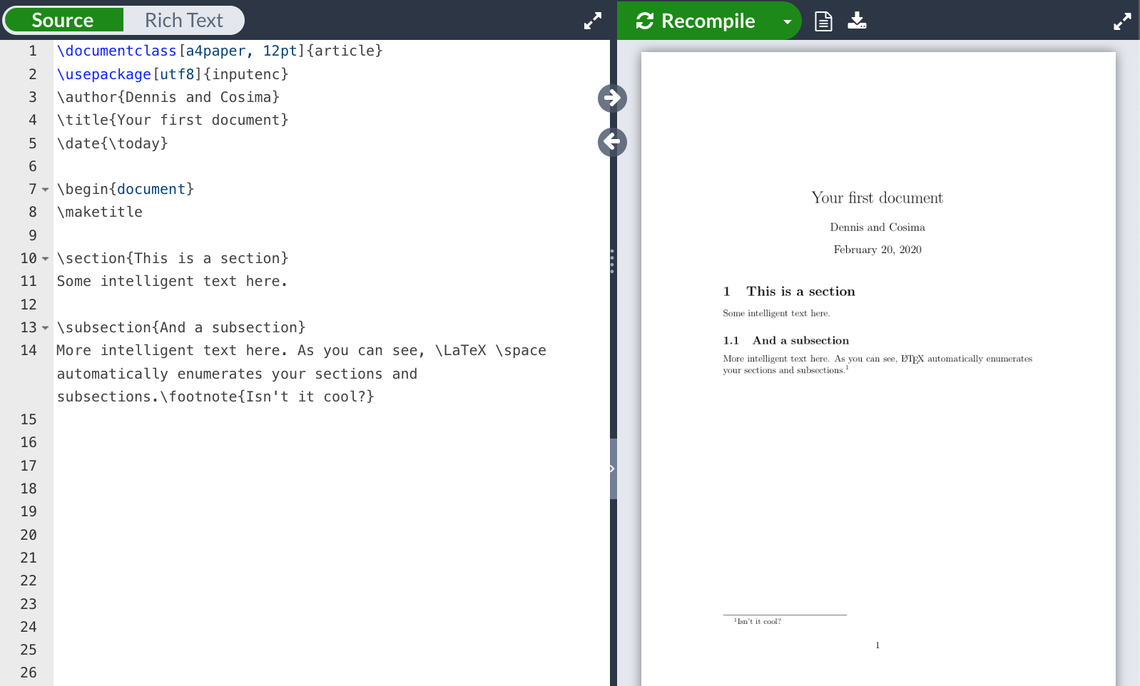
Before we explore LaTeX for automated and efficient (academic) writing, there are two important peculiarities of LaTeX to note. The first one is line breaks.
Compared to line breaks in other typesetters such as Word, where a new line starts after hitting ENTER, LaTeX requires you to be more specific. Most commonly, \\ is used to indicate a line break and usually follows right after the end of your text. Alternatively, you can also use ENTER twice in Overleaf to have one empty line in-between the text to produce a line break. Note, however, that several empty lines do not result in an equivalent number of line breaks. No matter how many empty rows are between one sentence and the next, LaTeX only gives you one single line break. To have more than one line in-between your text, you need to specify this explicitly, e.g., using \newline or specify \vspace{...} which allows you to define the exact length of the white space (\vspace{2cm}).
Another peculiarity, but also one of LaTeX and WYSIWYM’s main strengths, is that you can enter comments right in your body. All text after % is interpreted as a comment and will turn green in Overleaf (the color may change if you use another LaTeX editor). Comments do not show up in your final document but are still visible in the body of your .tex file. This is especially useful when you want to add notes to your document that should be shown in your final output, e.g., some small sub-headings that summarize the following paragraph or to-dos that are placed at specific sections of your paper. Moreover, comments can help you to quickly comment out text or even paragraphs that you do not want to lose but might not need at this time to show up in your final document, e.g., a literature section when you want to submit only your empirics part. This also helps to get rid of the (in)famous “Rest.docx” document that contains all leftovers that could eventually become important. We will explore this feature in more detail when we introduce our template below.
Taking Advantage of the Environment Structure in LaTeX
No matter what type of document you are producing, be it an academic article or a summary of thoughts, you almost always want to include things other than plain text. Of course, LaTeX allows you to include important aspects of documents such as lists, equations, figures, or tables as well. All of these additions to plain text can be added in the body at the exact position where you want them to be. For this, you take advantage of the environment structure in LaTeX. This means that we wrap a \begin{...} and an \end{...} around the respective object we want to include (e.g., a list, an equation, or a figure) and define everything within this environment. You can think of this as an environment that separates your text from other input and allows you to have specific modifications that only hold for this specific environment without affecting the rest of your text, e.g., to format the text within the environment into a list as outlined below.
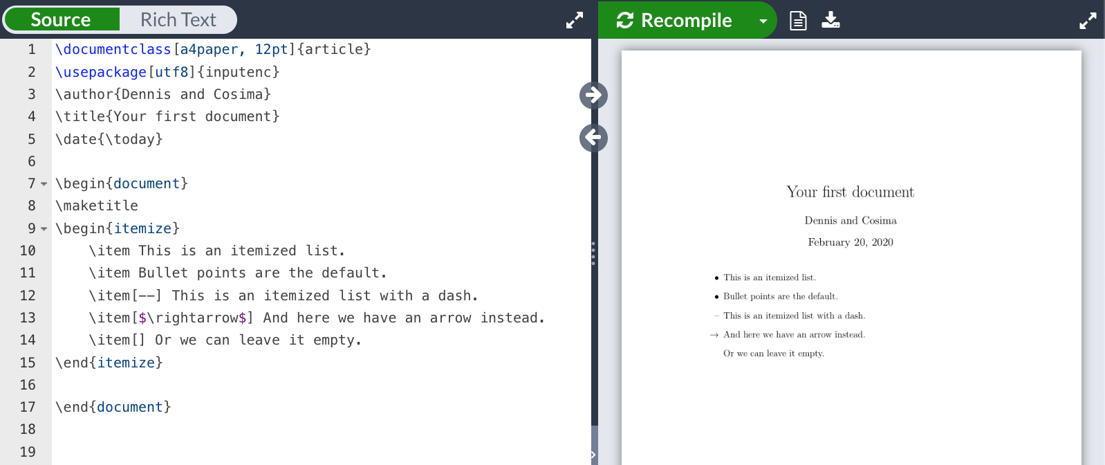
Creating lists
LaTeX offers two types of lists: itemized and enumerated lists. For itemized lists, you specify itemize in the beginning and at the end of your environment. Overleaf has a nice drop-down menu for specific environments and automatically provides you with the most basic set-up of the environment you have selected. Within the list environment, all text that follows after \item is now one bullet point in your list; more \item commands thus produce more bullet points with the respective text afterwards. Using squared brackets for each \item, you can modify the appearance of the bullet points, for instance to have a dash or an arrow. Note that using $...$ allows you to specify symbols from the math environment (more details below) that increases your variety of symbols for your lists. Leaving the squared brackets empty removes all symbols from the list, as you can also see in our example below.
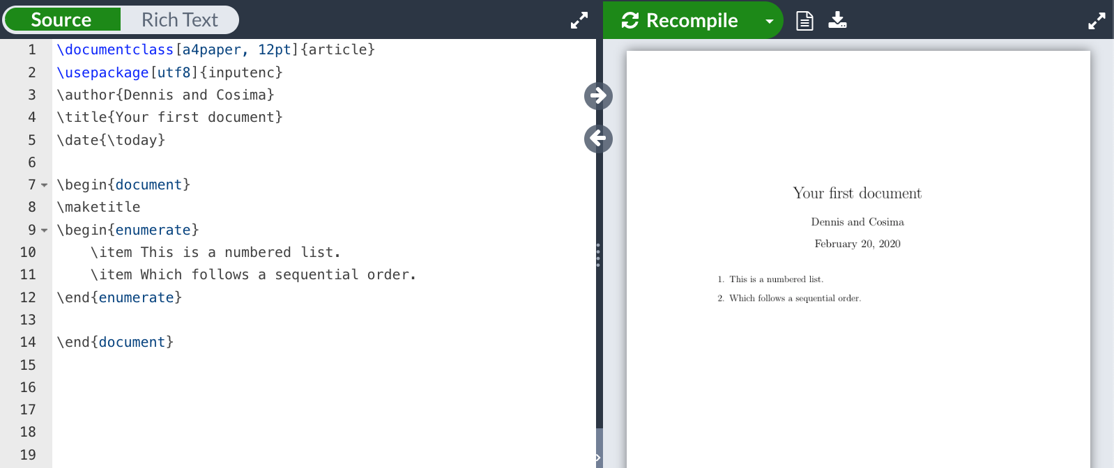
Enumerated lists follow the same logic as itemized lists. Even though you specify enumerate instead of itemize in the environment, you still use \item for each new entry in your list. By default, LaTeX enumerates a list using numbers in the form of 1. 2. 3. etc. For specific enumerated lists such as those with a) b) or c), there are packages such as enumitem.
Figure: Enumerated lists
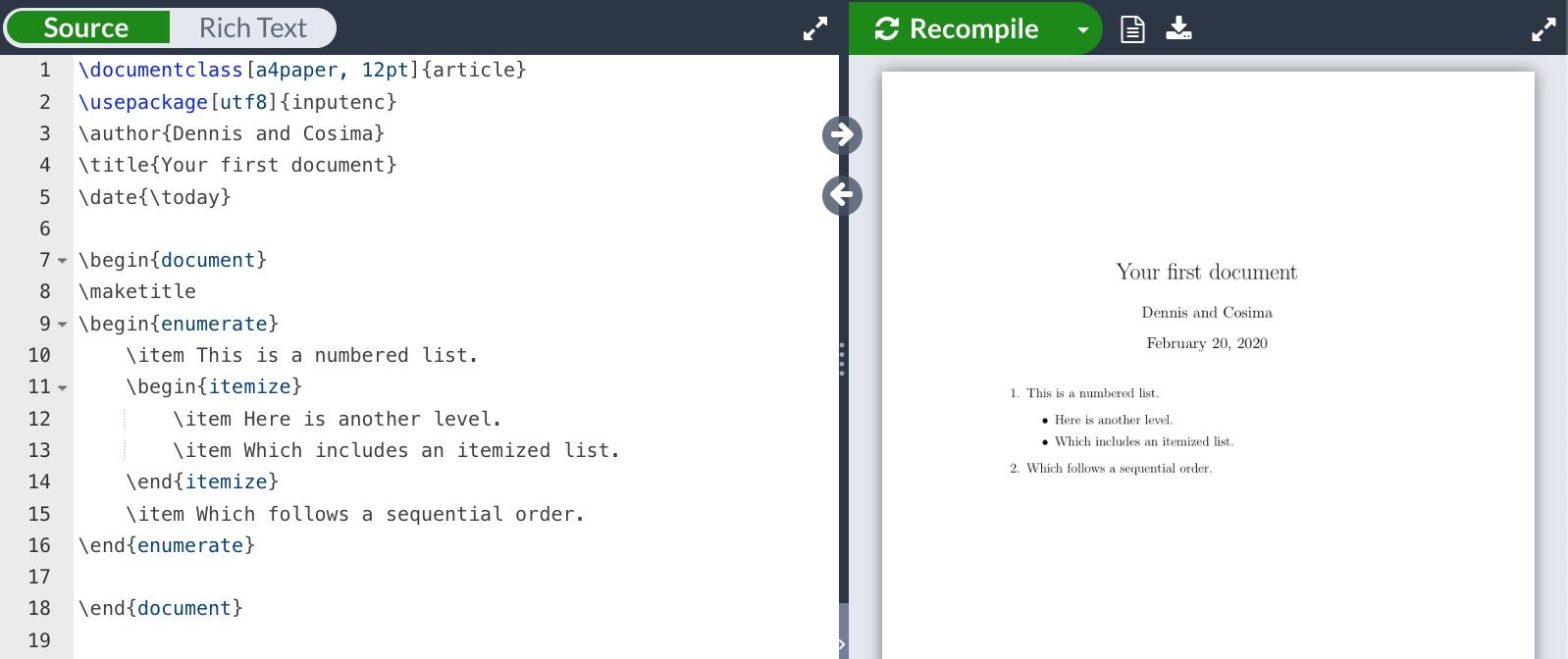
Both itemized and enumerated lists also allow you to create nested lists. You simply include another list environment to add another level to your list. LaTeX further allows you to mix and match enumerated and itemized lists here.
Figure: Nested lists
Equations
There are many ways to write equations in LaTeX. For simplicity, we only discuss two of the most common ways here. The first one is primarily used to include mathematical symbols or short equations within your written text. You have already seen this approach above: Without defining a separate environment, you can write your equation or math symbol within $...$. Math symbols in LaTeX are a world of its own and far too much to be covered in detail here. To get a basic idea of how to write equations and what symbols are available, see here.
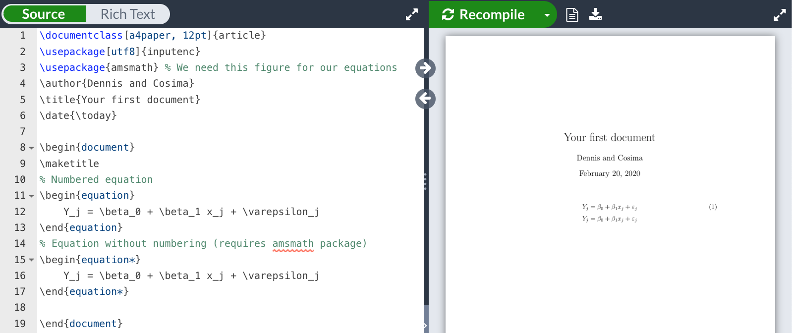
Standalone equations, i.e., those that start in a separate line and are enumerated, require the \begin{equation} ... \end{equation} environment. Similar to lists, the environment logic here separates your equation from the main text and allows you to modify different aspects of the equation.
The equation environment gives you, by default, a numbered equation; you can hide the enumeration by adding a * to your command (\begin{equation*} ... \end{equation*}) and loading the package amsmath in the preamble.
Figures
LaTeX also allows you to include figures in your document using the figure environment where you can easily pre-define all formatting for the output of your figure. To insert a figure in your document, you need to load the package graphicx in your preamble.
Again, in the well-known manner, we define a \begin{figure}...\end{figure} environment. To include the figure itself, you need to specify \includegraphics{...} in the figure environment with the figure name in curly brackets. Make sure that you provide the correct path to the figure in the curly brackets when working on your local machine or make use of Overleaf’s cloud-based storage. In Overleaf, you can upload files to your project using the sidebar. To add a caption, simply type \caption{...} below – or above \includegraphics{...} if you want the caption to appear above the figure. You may also want to center the figure by including \centering.
Luckily, Overleaf does all this for us by automatically inserting all relevant components of the figure environment. In addition, Overleaf also inserts a \label{...} that makes cross-referencing to your figure in the text possible. For instance, using the label \label{fig:logo}, you can refer to your figure anywhere in your text using \ref{fig:logo}. Cross-referencing also works with other objects that you enter, such as tables, or even footnotes, sections, and subsections.
The main advantage of using labels to cross-reference is that LaTeX, similar to footnotes, automatically updates the numbering of your figures in the cross-references according to their position. In other words, moving a figure below another one will automatically adjust the cross-reference in the output, e.g., from Figure 1 to Figure 2, as long as you keep the label in your figure the same.
Figures, as compared to lists or equations, usually float with the text in LaTeX unless defined otherwise. This means that LaTeX tries to put the figure where you have originally placed it unless there are space limitations or other restrictions. If this is the case, LaTeX chooses the best-fitting spot itself. Sometimes, this can be very useful but oftentimes you want to prevent LaTeX from rearranging your figures freely. To do so, you can add htpb! to the environment using squared brackets.
Tables
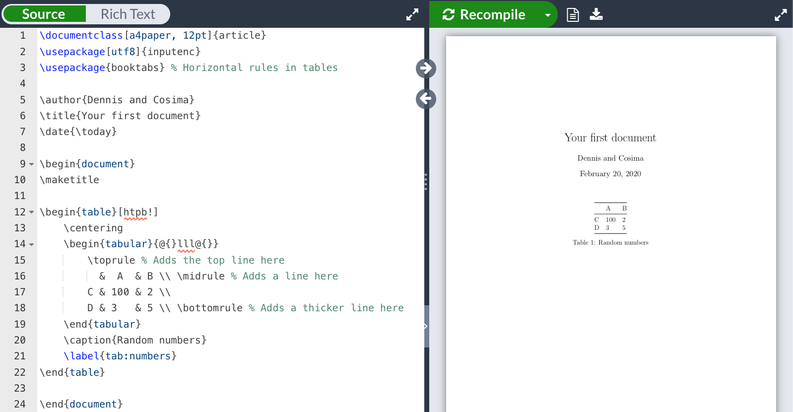
In contrast to lists or figures, tables are rather unintuitive and therefore among the more challenging objects in LaTeX. Fortunately, online table generators such as tablesgenerator.com are here to do the messy work of writing your own table for you. Tables are again defined in an environment: With \begin{table} ... \end{table} we are free to format the table with \centering, \caption{...}, and \label{...} as you have already seen with figures. To actually produce the table, however, we need to call another environment: \begin{tabular} ... \end{tabular}. You can basically think of the tabular environment as the equivalent of \includegraphics{...} for tables, only that you (or a table generator) need to construct the table yourself from scratch. We will not go into much detail about the specific logic of tables in LaTeX and recommend an online table generator where you have a pre-defined table setting and only insert your text in the table and let the online tool generate the LaTeX code for you. If you work in R and want to add your regression tables to your LaTeX document, there are various packages in R that generate a LaTeX formatted table based on your regression output (e.g., stargazer).
For a very simplistic outline of tables, the following table illustrates the basic logic. Columns are separated by & and rows by \\. Since horizontal lines in tables are common in scientific papers, using the package booktabs is recommended. This package allows you to use the commands \toprule, \midrule, and \bottomrule as seen below to specify horizontal lines.
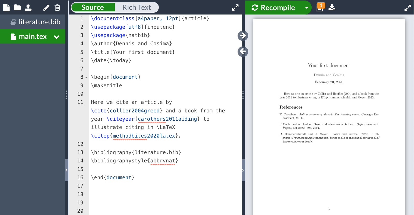
Citing in LaTeX
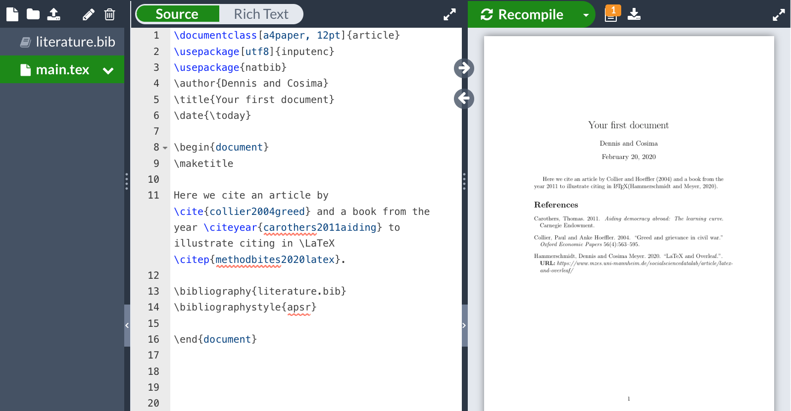
Another strength of LaTeX is its ability to generate automatic citations and bibliographies using packages such as natbib or bibtex, among others. To illustrate how to quickly set up citations, we use natbib in the following. This is also the package that is pre-installed in the template discussed below.
There are two main components to citations in LaTeX. The first one is a .bib file that contains all bibliography entries in a standardized format (see some examples below).
Citation managers such as Citavi, Mendeley, or Zotero can autmatically generate so-called BibTeX including all your library entries. Alternatively, you can retrieve them from Google Scholar using the citation button. In Overleaf, the .bib file is usually stored in your main directory and called at the end of your document using \bibliography{...}.
@article{collier2004greed,
  title={Greed and grievance in civil war},
  author={Collier, Paul and Hoeffler, Anke},
  journal={Oxford Economic Papers},
  volume={56},
  number={4},
  pages={563--595},
  year={2004},
  publisher={Oxford University Press}
}

@book{carothers2011aiding,
  title={Aiding democracy abroad: The learning curve},
  author={Carothers, Thomas},
  year={2011},
  publisher={Carnegie Endowment}
}

@online{methodbites2020latex,
  title={LaTeX and Overleaf},
  author={Hammerschmidt, Dennis and Meyer, Cosima},
  year={2020},
  url = {https://socialsciencedatalab.mzes.uni-mannheim.de/article/latex-intro/}
}
Each entry in your .bib file has a unique citation key at the beginning, e.g., methodbites2020latex. This will be used for your in-text citation. In order to cite an article or a book in your text, you only need to call \cite{...} with the unique citation key of your article as the input. Modifications such as page numbers can be inserted using squared brackets between your cite command and the citation key in the curly brackets. The list below provides an overview of different in-text citation styles.
The second main component is \bibliographystyle{...}. This modifies the appearance of your citation and bibliography according to specific citation styles. There are many popular citation styles already pre-loaded in natbib, such as apsr or abbrvnat. This is what you also see in the figure below. You can, of course, upload and add other citation styles that you find online as a .sty file to your directory in Overleaf. We, however, recommend – if possible – to use one of the default citation styles in Overleaf. Below is a short overview of how the appearance of citations change with different citation styles.
| Cite authors in-text (e.g., Collier and Hoeffler (2004)) |
\cite{...} or \citet{...}
|
| Cite author in parentheses (e.g., (Collier and Hoeffler, 2004)) |
\citep{...}
|
| Cite authors in-text (e.g., Collier and Hoeffler 2004) |
\citealt{...}
|
| Only cite authors names (e.g., Collier and Hoeffler) |
\citeauthor{...}
|
| Only cite the year (e.g., 2004) |
\citeyear{...}
|
| Cite a specific page (e.g., Collier and Hoeffler (2004, 4)) |
e.g., \cite[4]{...}
|
Figure: Citations
LaTeX Template: A Hands-on Guide
All the features outlined above – and many more – are nicely packaged in a ready-to-use template for (academic) writing in LaTeX and made accessible on Overleaf. The purpose of the template is to allow both beginners and more advanced LaTeX users to have a good starting point for writing their research papers in an automated and efficient workflow. It also contains special features that allow students to explore writing their term papers using LaTeX and thereby builds an ideal complement and resource for teaching.
The template further includes various options that can be customized (e.g., cover page/no cover page; including/excluding table of content, list of figures/tables) and provides a quick introduction into the very basics of LaTeX discussed above such as highlighting, citing, writing, including tables, figures, and mathematical equations.
What Does the Document Look Like?
The template encapsulates all aspects of an empirical term paper as well as those of almost all empirical academic studies. It comes with an organized folder structure that provides a good overview of the different text parts and helps to focus your writing process by only editing the text part that you want to focus on. In academic writing, documents usually consist of different sections, such as introduction or analysis. To organize these sections and to provide the user with a well-structured document outline, the LaTeX template we will discuss takes advantage of a well-organized folder structure and a clean outline of each section. For instance, if you want to work on your analysis, you only need to open the 6-analysis.tex file instead of having to scroll through the entire document and find the analysis section of your paper.
Following the distinction of LaTeX files into preamble and body, the template has a separate file called general.tex – that contains all necessary information for the preamble (packages, citation system, etc.) – and stores the written input of the document in a folder called “content”. In the content folder, each section of the paper has its own .tex file. These .tex files are dedicated to each section and can be fully customized. As they will be ensembled together and called within the \begin{document}...\end{document} environment of the main.tex file, they do not have a separate \begin{document}...\end{document} structure.
Figure: What’s in the “content” folder?
In order to bring our preamble and the body together, we use the main.tex file. This file follows our well-known structure and is separated into a preamble and a body. In the preamble section, we load the general.tex file and in the body all required sections of our paper that are stored in the “content” folder. Using this structure helps to quickly focus on a specific section of the paper by opening the associated .tex file for the section you are currently working on.
As you can see, we call the associated .tex files with \input{...} and their respective paths. This allows you also to only output those sections that are currently relevant to you by quickly commenting out the other sections with a % sign. Even though the output document has only those sections included that are not commented out, you still do not lose the text or the structure of your entire document. We showcase this by excluding the abstract. To do so, we comment out \input{content/1-abstract} with a % sign. As you can see, it will not appear in the paper anymore.
Figure: Commenting out sections
How to Use the Template and LaTeX for Your Research?
This blog post is intended as a first starting guide and a source for quick references for the basic usage and workflow of academic writing in LaTeX using a ready-to-use template. Naturally, the world of LaTeX is much larger and offers uncountable numbers of options, additions, packages, and modifications to explore. The template that is introduced here offers a starting point for both beginners and more advanced users of LaTeX.
For beginners, it summarizes all basic elements of LaTeX, including the structure of a general .tex document, introduction to text formatting as well as most commonly used environmental structures such as figures or equations. More advanced or curious users are able to explore the automated workflow that LaTeX provides using an organized folder structure and specific files for different tasks and purposes.
Both the template and the blogpost are thus intended to complement and hopefully advance academic writing as well as to provide a resource for teaching at the university and beyond.
Further Readings (and Help)
To explore the LaTeX universe even further, here are some general and more advanced guides:
- More simple template (similar to the one we used during the tutorial)
- Cheat sheet for LaTeX
- 30-minutes tutorial
- General tutorials
- To get an idea of LaTeX
- More templates
- Online table generator to create tables online
- List with mathematical expressions and a further reading of maths and equations in LaTeX
- If you are lost: Stack Exchange, Stack Overflow, and of course Google are always a good starting point
About the Presenters
Dennis Hammerschmidt is a doctoral researcher and lecturer at the University of Mannheim. He works at the intersection of quantitative methods and international relations to explore the underlying structure of state relations in the international system. Using information from political speeches and cooperation networks, his dissertation work analyzes the interaction of states at the United Nations and estimates alignment structures of states in the international arena.
Cosima Meyer is a doctoral researcher and lecturer at the University of Mannheim and one of the organizers of the MZES Social Science Data Lab. Motivated by the continuing recurrence of conflicts in the world, her research interest on conflict studies became increasingly focused on post-civil war stability. In her dissertation, she analyzes leadership survival – in particular in post-conflict settings. Using a wide range of quantitative methods, she further explores questions on conflict elections, women’s representation as well as autocratic cooperation.