Using Geospatial Data in R
The use of geospatial data – data that can be mapped using geographic information systems (GIS) – has become increasingly widespread in the social sciences. Applications not only extend to the analysis of classical geographical entities (e.g., policy diffusion across spatially proximate countries) but increasingly also to analyses of micro-level data, including respondent information from georeferenced surveys or user trace data from Tweets. In this Methods Bites Tutorial, Stefan Jünger (GESIS) and Denis Cohen (MZES) show how to retrieve, manage, and visualize geospatial data in R.
After reading this blog post and engaging with the applied exercises, readers will be able to:
- retrieve geospatial data from Open Street Map and other sources
- perform data wrangling with simple features (a geospatial data format)
- visualize geospatial information using 2D and 3D maps
Note: This blog post builds up on Stefan’s workshop Management and Analysis of Georeferenced Survey Data in the MZES Social Science Data Lab. The original workshop materials, including slides and scripts, are available from our GitHub. A live recording of the workshop is available on our YouTube Channel. Additional learning materials on this topic are linked in the Further Reading section below.
Overview
Geospatial data: An overview
Geospatial data comprise information about geometries (points, lines, polygons, grids) related to a location on a map. This relation is usually established through coordinate data – so-called geo-coordinates, which carry information on longitude and latitude.1 These geo-coordinates are projected onto the earth’s surface, where we can use them to represent any geometry (see the figure below). For instance, a specific location can be represented by a point using a coordinate pair for the locations longitude and latitude. Roads or rivers can be represented by a linestring, i.e., a connected sequence of such points. Areas, such as the layouts of buildings or the boundaries of neighborhoods, municipalities, counties, or countries, can be represented by polygonal shapes. Lastly, grid cells can be used to provide spatial summaries of variables such as population density or the proportion of ethnic minority residents in small artifical square areas (e.g., square kilometer grid cells). Geospatial data is georeferenced, meaning that direct spatial identifiers in the form of geo-coordinates can reference any point on earth.
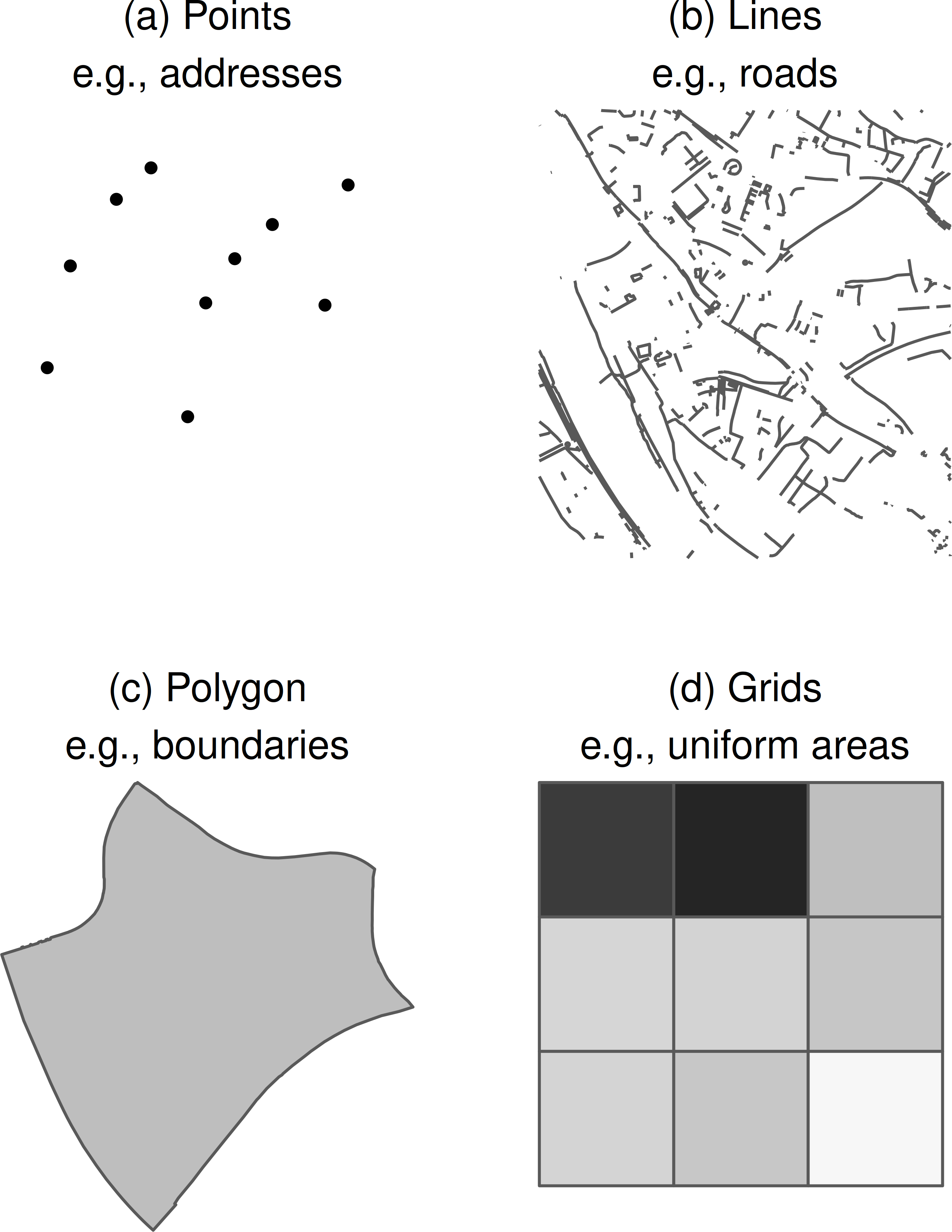
Source: Jünger (2019)
There is, however, one big issue with this referencing. Since our earth is three-dimensional and maps are only two-dimensional, projection of points comes with the price of distorting geometries upon display. One of the most prominent systems of projection is the Mercator projection used for navigation purposes. Within this projection, geometries on the edge of a world map are usually represented bigger than they are. You can find an excellent interactive visualization of this issue here. For such reasons, there are different projection systems or Coordinate Reference Systems (CRS), which can be used for various purposes. We will not go into detail here, but we need to know that whenever we aim to link different geospatial data sources, their respective CRS must match.
The idea of using geospatial information in the social sciences is not particularly new. For decades, researchers have considered the role of individuals’ geo-social context (e.g., neighborhoods) when explaining individual behaviors or attitudes. Many theories also implicitly or explicitly incorporate space into their fundamental assumptions. For example, Allport’s (1954) Contact Theory, which explains prejudice by the frequency of everyday interactions between members of ingroups and outgroups, is fundamentally based on the idea of spaces or places where people eventually meet. As such, the relevance of and motivations for using geospatial information should not be too alien for scholars of social behavior.
What has changed during the last decades, however, is the sheer amount of resources we can exploit for research on the repercussions of geospatial contexts on social behavior, both computationally and with respect to data availability. Accordingly, the set of social science applications is diverse, ranging from work in the field of social inequalities (Panzera and Postiglione 2020), environmental justice (Rüttenauer 2019), conflict research (Oswald, et al. 2020), to health (Greiner et al. 2018).
Data retrieval and data management
Geospatial data can be big as big data. Millions of geometries, such as points, are no exception, making working with geospatial data quite demanding. Today’s personal computers are capable of processing large data sets; however, retrieving geospatial data still requires smart and flexible methods of loading and accessing the data. Therefore, we often rely on Web Services and Application Programming Interfaces (API) to access data, such as OpenStreetMap’s Overpass API, which are helpful to load only the chunks of data we are interested in using. Only seldom we need access to all data at once.
Still, geospatial data comes in different formats, and it is dependent on the task of which format is best suited for further processing. Raster data (see the Census example below) is great for areal data that do not differ between each geometry. Vector data is perfect for data that may comprise similar geometries, such as lines, but whose shapes vary. In the applied examples below, we will leverage both data types, but vector data in particular needs a closer look since we will use the excellent implementation of simple features in R for that purpose that we will introduce now.
What are simple features?
First and foremost, simple features comprise a file format for geospatial vector data, following the ISO 19125-1:2004 standard. The name in itself can be seen as a nickname, but the term also says it all: simple features are relatively easy to handle. Their implementation in R as developed in the sf package has enormous advantages compared to more traditional file formats for geospatial data in R2:
- They depict a flat-file structure: Any
sfobject is basically a rectangular table with features (i.e., observations or geometries) in the rows and attributes or variables in the columns. - The only difference to other rectangular data is a so-called
geometrycolumn that defines each features’ geometry (point, lines, polygons, etc.). These may be supplemented with metadata, e.g., a definition the coordinate reference system of the geospatial data. - A lot of techniques in the
sfpackage which rely on the file format can be perfectly integrated in a tidyverse workflow using pipes (%>%) ordplyrverbs.
Please refer to this great resource on simple features in R if you are interested in more specifics of the data format.
Gathering geospatial data
To gather geospatial data, we use the osmdata package. This package facilitates the download of OpenStreetMap (OSM) data by providing a straightforward syntax for OSM data quires from the Overpass API. OSM is a community-driven open-access project for mapping geographical data. osmdata allows for the direct import of OSM data as sf objects. This makes it easy to collect and combine various layers of data and to use the data in conjunction with other R packages for the management, analysis, and visualization of geospatial data.
In the following, we illustrate the use of sf objects retrieved from osmdata queries by walking readers through the generation and visualization of a data set on streets, buildings, and population characteristics in Mannheim.
Readers who would like to run these applications on their own machines should have the following packages installed:
Code: R packages used in this tutorial
## Save package names as a vector of strings
pkgs <- c("dplyr", "ggplot2", "ggnewscale", "ggsn", "osmdata", "sf", "z11")

## Install uninstalled packages
if (!("z11" %in% installed.packages()))
  remotes::install_github("StefanJuenger/z11")
lapply(pkgs[!(pkgs %in% installed.packages())], install.packages)

## Load all packages to library and adjust options
lapply(pkgs, library, character.only = TRUE)
Mannheim’s boundaries from OpenStreetMap
We start by retrieving a boundary box that includes all of Mannheim’s area. We specify the requested boundaries using osmdata::getbb() and initialize the Overpass query using osmdata::opq().
The function osmdata::add_osm_feature() allows us to retrieve administrative boundaries (specified by key = "admin_level") within our boundary box at the municipal level, defined by the value argument. osmdata::osmdata_sf() ensures that the retrieved data is imported as an sf object.
In additional processing steps, we extract the polygon data of the administrative boundaries in our boundary box and filter those boundaries which belong to Mannheim (as opposed to neighboring cities and municipalities). We do this by defining a filter which selects only polygons associated with the city name. From our experience, it’s always a good idea to use the country’s language for the city name. Lastly, we select the polygon geometry information and convert the GIS coordinates to a specific coordinate reference system (CRS) using sf::st_transform(3035).
mannheim <-
  osmdata::getbb("Mannheim") %>%
  osmdata::opq(timeout = 25*100) %>%
  osmdata::add_osm_feature(
    key = "admin_level",
    value = "6"
  ) %>%
  osmdata::osmdata_sf() %$%
  osm_multipolygons %>%
  dplyr::filter(name == "Mannheim") %>% # filter on city level
  dplyr::select(geometry) %>%
  sf::st_transform(3035)

mannheim
## Simple feature collection with 1 feature and 0 fields
## geometry type: MULTIPOLYGON
## dimension: XY
## bbox: xmin: 4206252 ymin: 2923007 xmax: 4218767 ymax: 2943155
## projected CRS: ETRS89-extended / LAEA Europe
## geometry
## 1 MULTIPOLYGON (((4209130 293...We can see that the resulting data is essentially a raw data table that comprises some metadata, such as the CRS. Thus, we can use standard data wrangling techniques in R. For instance, we can simply plot the boundary data using ggplot2’s geom_sf(). This gives us an otherwise empty shading of Mannheim’s boundaries:
ggplot(mannheim, fill = NA) +
  geom_sf() +
  ggsn::blank()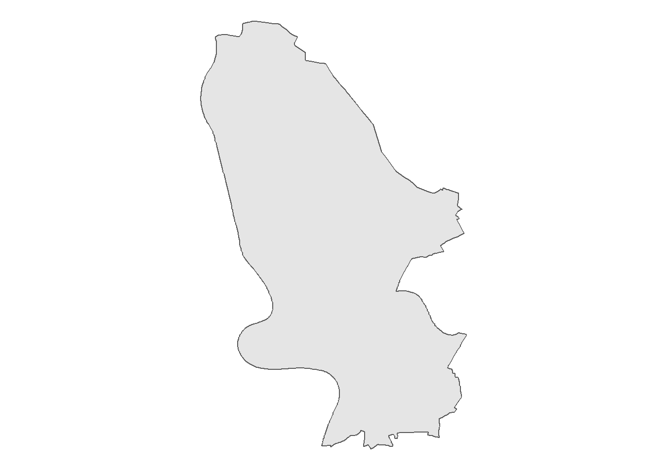
Adding data: Streets, buildings, and foreign-born residents
To fill this map with life, we gather additional data from OpenStreetMap. We start by retrieving additional geometries for streets and roads, which we store in the object roads. Our query is vastly similar to our initial one. Of course, the main difference is that we now request different features in osmdata::add_osm_feature(). As opposed to retaining polygonal data via osm_multipolygons, we now request lines depicting streets and roads via osm_lines.
Lastly, we retain only those street and road data that intersect with the administrative boundaries of Mannheim and make sure that we keep linestring geometries only.
roads <-
  osmdata::getbb("Mannheim") %>%
  osmdata::opq(timeout = 25*100) %>%
  osmdata::add_osm_feature(
    key = "highway",
    value = c(
      "trunk",
      "primary",
      "secondary",
      "tertiary"
      )
  ) %>%
  osmdata::osmdata_sf() %$%
  osm_lines %>%
  dplyr::select(geometry) %>%
  sf::st_transform(3035) %>%
  sf::st_intersection(mannheim) %>%
  dplyr::filter(
    sf::st_is(., "LINESTRING")
    )
Next, we proceed similarly for data on a various types of buildings (specified per the value argument in osmdata::add_osm_feature()). As buildings have two-dimensional areal footprints (as opposed to roads, which can be represented by simple lines), we once again extract osm_polygons and retain only those buildings that intersect with the administrative boundaries of Mannheim.
buildings <-
  osmdata::getbb("Mannheim") %>%
  osmdata::opq(timeout = 25*100) %>%
  osmdata::add_osm_feature(
    key = "building",
    value = c(
      "apartments", "commercial",
      "office", "cathredral", "church",
      "retail", "industrial", "warehouse",
      "hotel", "house", "civic",
      "government", "public", "parking",
      "garages", "carport",
      "transportation",
      "semidetached_house", "school",
      "conservatory"
    )
  ) %>%
  osmdata::osmdata_sf() %$%
  osm_polygons %>%
  dplyr::select(geometry) %>%
  sf::st_transform(3035) %>%
  sf::st_intersection(mannheim)
Lastly, we add data on the geospatial density of Mannheim’s foreign-born population. Toward this end, we use processed data from the 2011 German Census, aggregated at a geospatial raster of 1 sqkm grid cells. This data is available from Stefan’s z11 package. The variable itself is a standard measure for ethnic diversity, e.g., to investigate Allport’s hypothesis that contact between people of different groups reduces prejudices (Klinger et al. 2017). It also is helpful in inequality research when assessing whether foreign-born residents are, for example, more exposed to environmental hazards (Rüttenauer 2019).
We transform the raster data to sf-readable polygon data using the same CRS as before. This means that each 1 sqkm grid cell can now be plotted onto our existing map of Mannheim per the geometry information in foreign_born whereas the variable layer in foreign_born stores the percentage of foreign-born residents in each grid cell.
foreign_born <-
  z11::z11_get_1km_attribute(Auslaender_A) %>%
  raster::crop(mannheim) %>%
  raster::rasterToPolygons() %>%
  sf::st_as_sf() %>%
  sf::st_transform(3035) %>%
  sf::st_intersection(mannheim) %>%
  dplyr::filter(layer > -1)
Data visualization
2D plots
Now that we have gathered all the data that we would like to include in our illustration, the question is how to best present the different types of geospatial information. A straightforward solution would be presenting separate plots, e.g., one for streets and buildings and one for the density of Mannheim’s foreign-born population. However, separating information across numerous plots makes it hard to relate information from different variables to one another. An alternative approach, shown below, involves flattening multiple data layers, i.e., collapsing many geospatial variables onto a single two-dimensional map.
This is easy enough to do in the current example, where coarse areal mappings (grid cells) are supplemented with much finer areal (buildings) and linear (streets) data. However, even the addition of one additional layer with coarse areal information – e.g., additional census information on the percentage of the senior population at the 1 sqkm grid cell level – would result in a visually indistinguishable overlay of information.
ggplot() +
  geom_sf(data = mannheim) +
  geom_sf(
    data = foreign_born,
    aes(fill = layer,
        alpha = 0.8),
    color = NA
  ) +
  scale_fill_distiller(
    palette = "Greens",
    direction = 1,
    guide = FALSE
  ) +
  geom_sf(data = roads) +
  geom_sf(data = buildings) +
  theme(legend.position = "none") +
ggsn::blank() 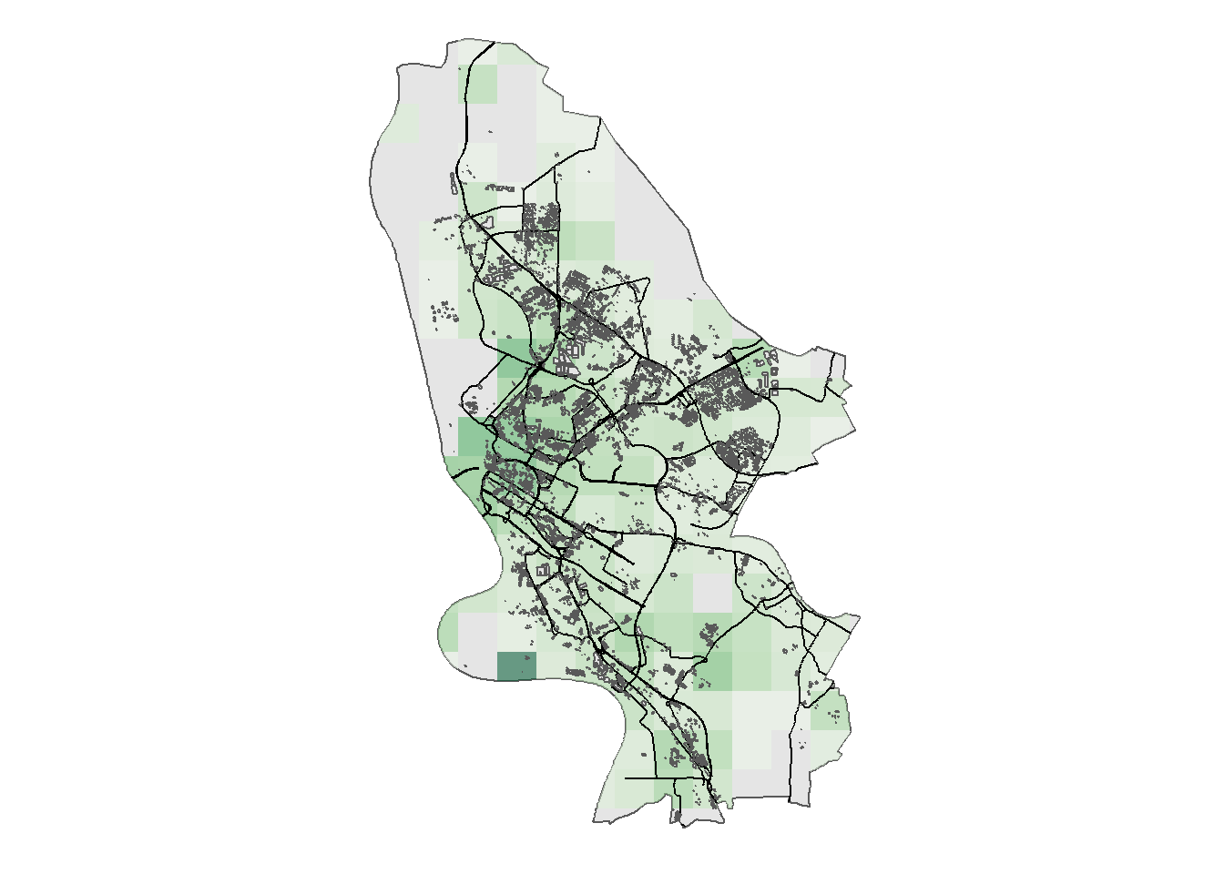
3D plots
An alternative to flattening multiple layers onto a two-dimensional map is using a three-dimensional vertical stacking of the layers. This allows us to show even large numbers of overlapping geometries in a single plot, which yields compact yet accessible visualizations of multiple pieces of geospatial information.
Mathematically, we can create such a map with shearing and rotating any point in our input data:
\[{[x,y]} \times \underbrace{\begin{bmatrix}2 & 0 \\ 1.2 & 1 \end{bmatrix}}_\text{Shear Matrix} \times \underbrace{\begin{bmatrix} \cos(\frac{\pi}{20}) & \sin(\frac{\pi}{20}) \\ -\sin(\frac{\pi}{20}) & \cos(\frac{\pi}{20})\end{bmatrix}}_\text{Rotation Matrix} \underbrace{(+ \begin{bmatrix}x\_add & y\_add \end{bmatrix})}_\text{Optional Additions}\]
We can also add an \(x\) or \(y\) offset value to move all points in two-dimensional space at the end of this operation.3
In order to use our sf data, stored in an inherently two-dimensional CRS, we need to devise an auxiliary function in R that allows us to shear and rotate these two-dimensional simple features such that they can be displayed in a three-dimensional space. It’s a basic and self-written implementation of the formula above.
Code: Defining the
rotate_sf() function
#' Rotate simple features for 3D layers
#' Rotates a simple features layer using a shear matrix transformation on the
#' \code{geometry} column. This can get nice for visualisation and works with
#' points, lines and polygons.
#'
#' @param data an object of class \code{sf}
#' @param x_add integer; x value to move geometry in space
#' @param y_add integer; x value to move geometry in space
#'
#' #' @importFrom magrittr %>%

rotate_sf <- function(data, x_add = 0, y_add = 0) {

  shear_matrix <- function (x) {
    matrix(c(2, 1.2, 0, 1), 2, 2)
  }

  rotate_matrix <- function(x) {
    matrix(c(cos(x), sin(x), -sin(x), cos(x)), 2, 2)
  }

  data %>%
    dplyr::mutate(
      geometry =
        .$geometry * shear_matrix() * rotate_matrix(pi / 20) + c(x_add, y_add)
    )
}
Now that the rotate_sf() function has been defined, we can use it to produce a figure that shows the information on streets and buildings in the base layer. On top of this base layer, we stack a semi-transparent raster that shows the density of the Mannheim foreign-born population.
ggplot() +
  geom_sf(data = rotate_sf(mannheim),
          fill = NA) +
  geom_sf(data = rotate_sf(roads)) +
  geom_sf(data = rotate_sf(buildings)) +
  geom_sf(data = rotate_sf(mannheim, y_add = 15000),
          fill = NA,
          color = "gray",
          alpha = 0.2) +
  geom_sf(
    data = rotate_sf(foreign_born, y_add = 15000),
    aes(fill = layer,
        alpha = .8),
    color = NA
  ) +
  scale_fill_distiller(palette = "Greens",
                       direction = 1,
                       guide = FALSE) +
  theme(legend.position = "none") +
  ggsn::blank()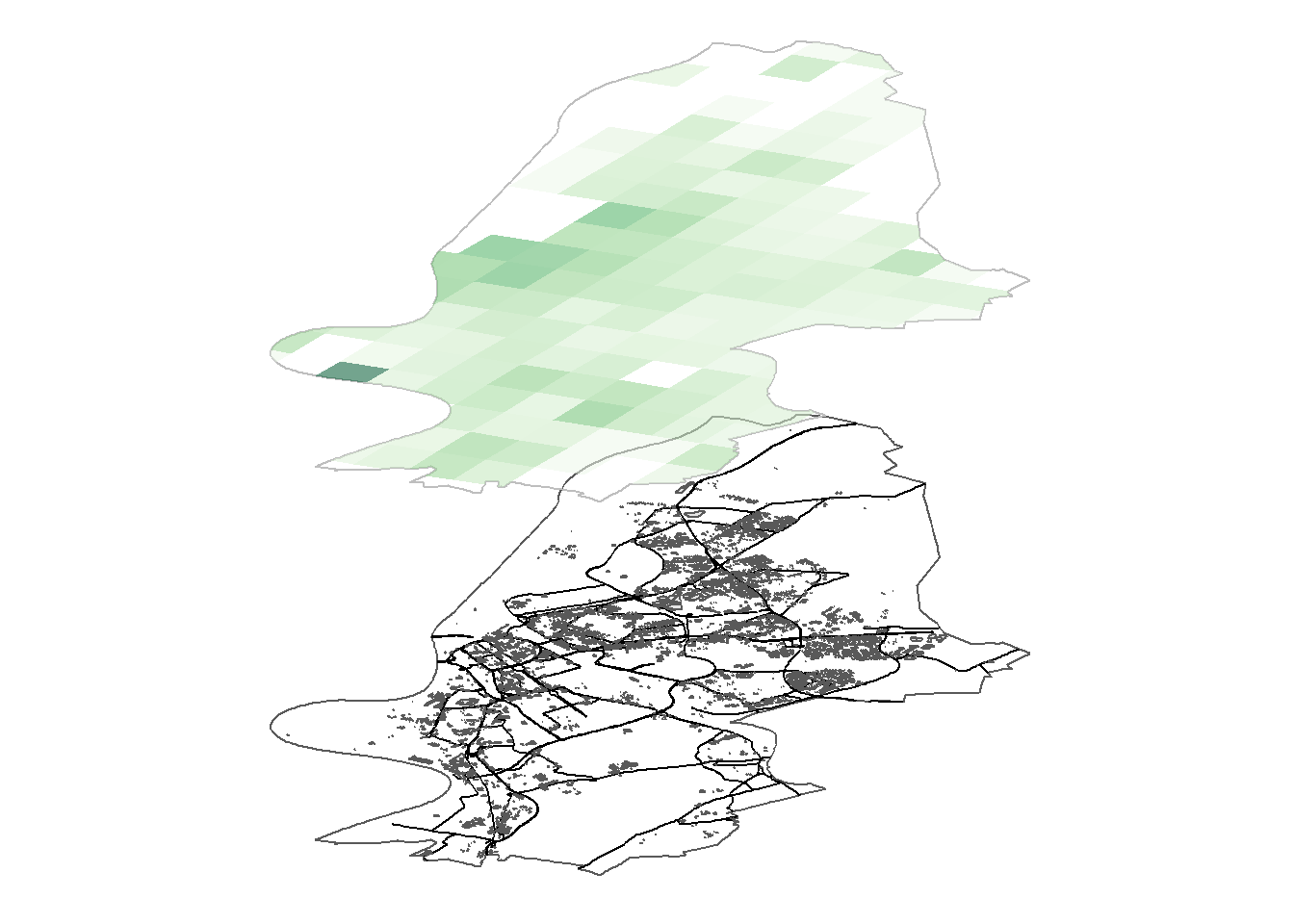
Below, we show how this idea can be extended by introducing the share of the senior (aged 65+) population at the 1 sqm grid cell level as an additional layer. The 3D display allows us not only to present information on both the foreign-born population and the senior population at once, but also to relate the two variables to one another. In other words, with the stacked 3D display, we can visually inspect the association between two or more variables. This is a unique asset of this type of three-dimensional visualization as there is no straightforward equivalent in a two-dimensional map.
Code: Adding another layer
## Retrieve data
seniors <-
  z11::z11_get_1km_attribute(ab65_A) %>%
  raster::crop(mannheim) %>%
  raster::rasterToPolygons() %>%
  sf::st_as_sf() %>%
  sf::st_transform(3035) %>%
  sf::st_intersection(mannheim) %>%
  dplyr::filter(layer > -1)

## Plot
ggplot() +
  geom_sf(data = rotate_sf(mannheim),
          fill = NA) +
  geom_sf(data = rotate_sf(roads)) +
  geom_sf(data = rotate_sf(buildings)) +
  geom_sf(
    data = rotate_sf(mannheim, y_add = 15000),
    fill = NA,
    color = "gray",
    alpha = 0.2
  ) +
  geom_sf(
    data = rotate_sf(foreign_born, y_add = 15000),
    aes(fill = layer,
        alpha = .8),
    color = NA
  ) +
  scale_fill_distiller(palette = "Greens",
                       direction = 1,
                       guide = FALSE) +
  new_scale_fill() +
  geom_sf(
    data = rotate_sf(mannheim, y_add = 30000),
    fill = NA,
    color = "gray",
    alpha = 0.2
  ) +
  geom_sf(data = rotate_sf(seniors, y_add = 30000),
          aes(fill = layer,
              alpha = .8),
          color = NA) +
  scale_fill_distiller(palette = "Reds",
                       direction = 1,
                       guide = FALSE) +
  theme(legend.position = "none") +
  ggsn::blank()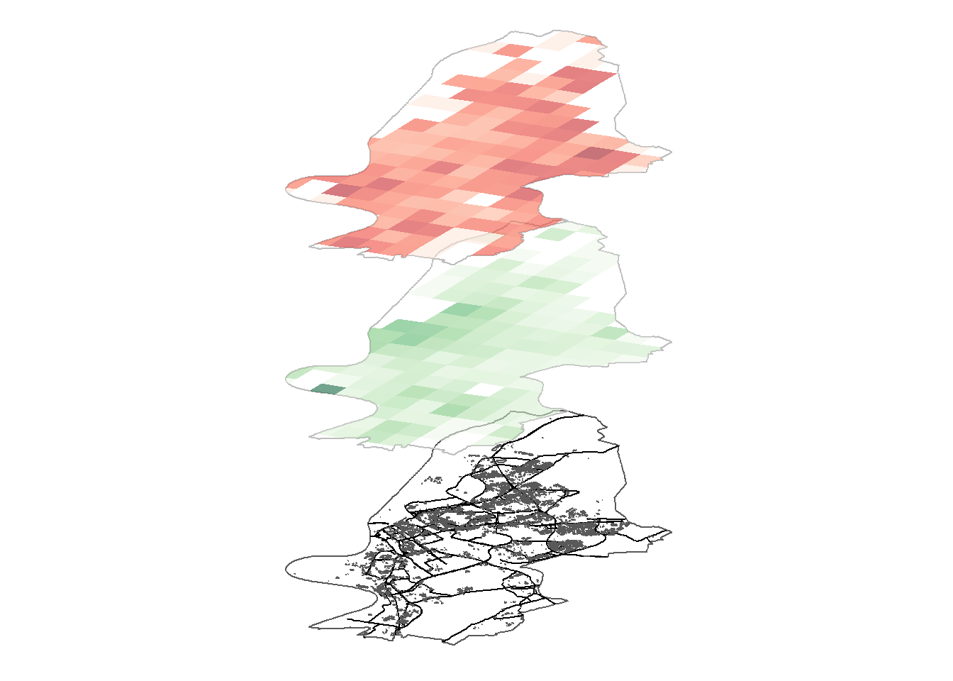
Conclusion
Geospatial data is being increasingly used in the social sciences, be it to study the relationship between various features of (partly) overlapping geographical entities, to study spatial correlation and spillover between proximate geographical entities, or to study context effects on micro-level attitudes and behavior. In this blog post, we have outlined core features of Geographic Information Systems and showcased tools for the retrieval, management, and uni-, bi-, and multivariate descriptive visualization of geospatial data in 3D. This workflow can take researchers a long way in working with geospatial data and constitutes an important step toward full-blown spatial data analyses.
References
- Allport, Gordan W. 1954. The Nature of Prejudice. Cambridge, Massachusetts: Addison-Wesley Publishing Company
- Greiner, Gregory Gordon, Schwettmann, Lars Goebel, Jan and Maier, Werner. 2018. Primary care in Germany: access and utilisation—a cross-sectional study with data from the German Socio-Economic Panel (SOEP). BMJ Open, 8(10), e021036
- Klinger, Julia, Stefan Müller, and Merlin Schaeffer. 2017. Der Halo-Effekt in einheimisch-homogenen Nachbarschaften: Steigert die ethnische Diversität angrenzender Nachbarschaften die Xenophobie? Zeitschrift für Soziologie 46 (6), 402–19
- Jünger, Stefan. 2019. Using Georeferenced Data in Social Science Survey Research. The Method of Spatial Linking and Its Application with the German General Social Survey and the GESIS Panel. Köln: GESIS - Leibniz Institute for the Social Sciences
- Oswald, Christian, et al. 2020. Under the roof of rebels: civilian targeting after territorial takeover in Sierra Leone. International Studies Quarterly 64.2, 295-305
- Panzera, Domenica and Postiglione, Paolo. 2020. Measuring the Spatial Dimension of Regional Inequality: An Approach Based on the Gini Correlation Measure. Social Indicators Research, 148(2), 379–394
- Percivall, George. 2016. OGC’s Open Standards for Geospatial Interoperability. In S. Shekhar, H. Xiong, & X. Zhou (Hrsg.), Encyclopedia of GIS (p. 1–7). Cham: Springer International Publishing
- Rüttenauer, Tobias. 2019. Bringing urban space back in: A multilevel analysis of environmental inequality in Germany. Urban Studies, 56(12), 2549–2567
- Simmons, Beth and Elkins, Zachary. 2004. The Globalization of Liberalization: Policy Diffusion in the International Political Economy. The American Political Science Review, 98(1), 171-189.
- Statistische Ämter des Bundes und der Länder. 2011. Zensus 2011 - Methoden und Verfahren
Further reading
- Bivand, Roger S., Edzer Pebesma, and Virgilio Gómez-Rubio. 2013. Applied Spatial Data Analysis with R. New York, NY: Springer New York.
- Jünger, Stefan. 2019. Using Georeferenced Data in Social Science Survey Research. The Method of Spatial Linking and Its Application with the German General Social Survey and the GESIS Panel. Köln: GESIS - Leibniz Institute for the Social Sciences
- Lovelace, Robin, Jakub Nowosad, and Jannes Münchow. 2019. Geocomputation with R. Boca Raton: CRC Press, Taylor and Francis Group, CRC Press is an imprint of theTaylor and Francis Group, an informa Buisness, A Chapman & Hall Book.
In spherical coordinate systems, this two-dimensional horizontal information may be supplemented with information on elevation or altitude.↩︎
This should, of course, not diminish the value of other formats. For instance,
SpatialPolygonDataFrameshave always been useful and still are great. However, these objects are deeply nested and thus sometimes difficult to handle. Operations using simple features are often also way faster.↩︎Shearing is a common concept in geometry. Don’t worry too much about the math here.↩︎
