Generalized Additive Models: Allowing for some wiggle room in your models
Generalized additive models (GAMs) have become an important tool for modeling data flexibly. These models are generalized linear models where the outcome variable depends on unknown smooth functions of some predictor variables, and where the interest focuses on inference about these smooth functions. In this Methods Bites Tutorial, Sara Stoudt (Smith College) offers a hands-on recap of her workshop “Generalized Additive Models: Allowing for some wiggle room in your models” in the MZES Social Science Data Lab in March 2021.
After reading this blog post and engaging with the applied exercises, readers should:
- be able to understand conceptually how GAMs relate to GLMs,
- be comfortable with the syntax of a
gammodel, - be aware of the tuning parameters within a “smooth”, and
- know what diagnostics are available to them.
Note: This blog post provides a summary of Sara’s workshop in the MZES Social Science Data Lab. The original workshop materials, including slides and scripts, are available from GitHub.
A live recording of the workshop is available on our YouTube Channel.
Overview
GAMs: a wiggly GLM
Have you ever wanted just a little more wiggle room in your models? You suspect that a covariate is not linearly related to the response on some scale, but rather has a curved relationship to the response. Then a generalized additive model is for you! A generalized additive model (or GAM) is just a more flexible generalized linear model.
To estimate GAMs, you need the following packages:
# For GAMs
library(mgcv)
# And to deal with the data
library(tidyverse)
library(lubridate)
And load the data:
data <- read.csv("https://raw.githubusercontent.com/sastoudt/MZES_GAMs/main/Data/dailyStops.csv")As a starting point, we will consider this generalized linear model of daily number of traffic stops (for more context on the data, go to the source). We get a different level per day of the week and let there be a linear trend across months.
generalized_linear_model <-
  glm(
    daily_num_stops ~ driver_race + post_policy + driver_race * post_policy + day_of_week + month,
    data = data,
    family = "quasipoisson"
  )
Output of
generalized_linear_model
summary(generalized_linear_model)##
## Call:
## glm(formula = daily_num_stops ~ driver_race + post_policy + driver_race *
## post_policy + day_of_week + month, family = "quasipoisson",
## data = data)
##
## Deviance Residuals:
## Min 1Q Median 3Q Max
## -26.916 -5.885 -1.194 4.269 38.670
##
## Coefficients:
## Estimate Std. Error t value Pr(>|t|)
## (Intercept) 5.551688 0.031241 177.707 <2e-16 ***
## driver_raceHispanic -1.997720 0.063874 -31.276 <2e-16 ***
## driver_raceWhite 0.698847 0.026995 25.888 <2e-16 ***
## post_policy 0.302333 0.028405 10.644 <2e-16 ***
## day_of_weekMonday -0.251005 0.028354 -8.852 <2e-16 ***
## day_of_weekSaturday 0.007252 0.026407 0.275 0.7836
## day_of_weekSunday -0.340416 0.029000 -11.738 <2e-16 ***
## day_of_weekThursday -0.360710 0.029269 -12.324 <2e-16 ***
## day_of_weekTuesday -0.347524 0.029152 -11.921 <2e-16 ***
## day_of_weekWednesday -0.265579 0.028472 -9.328 <2e-16 ***
## month -0.004370 0.002278 -1.918 0.0551 .
## driver_raceHispanic:post_policy 0.029594 0.081672 0.362 0.7171
## driver_raceWhite:post_policy -0.037925 0.034789 -1.090 0.2757
## ---
## Signif. codes: 0 '***' 0.001 '**' 0.01 '*' 0.05 '.' 0.1 ' ' 1
##
## (Dispersion parameter for quasipoisson family taken to be 67.57155)
##
## Null deviance: 998623 on 4378 degrees of freedom
## Residual deviance: 284627 on 4366 degrees of freedom
## AIC: NA
##
## Number of Fisher Scoring iterations: 5But it seems plausible that the number of traffic stops doesn’t just increase or decrease across months, but maybe fluctuates back and forth. Similarly, by fitting a different coefficient for each day of the week, we’re losing out on potential information, like we expect Monday to be more like Tuesday than Friday. That’s where GAMs (in the package mgcv) can help us.
data$day_of_week_num <-
  as.numeric(as.factor(data$day_of_week))

## now want to allow smoothness across days of week rather than
## a separate coefficient for each day

generalized_additive_model <-
  mgcv::gam(
    daily_num_stops ~ driver_race + post_policy + driver_race * post_policy +
      s(day_of_week_num, bs = "cc", k = 4) + s(month, bs = "cc"),
    data = data,
    family = "quasipoisson"
  )
Output of
generalized_additive_model
summary(generalized_additive_model)##
## Family: quasipoisson
## Link function: log
##
## Formula:
## daily_num_stops ~ driver_race + post_policy + driver_race * post_policy +
## s(day_of_week_num, bs = "cc", k = 4) + s(month, bs = "cc")
##
## Parametric coefficients:
## Estimate Std. Error t value Pr(>|t|)
## (Intercept) 5.30945 0.02275 233.336 <2e-16 ***
## driver_raceHispanic -1.99774 0.06577 -30.375 <2e-16 ***
## driver_raceWhite 0.69885 0.02780 25.142 <2e-16 ***
## post_policy 0.29755 0.02928 10.163 <2e-16 ***
## driver_raceHispanic:post_policy 0.02961 0.08410 0.352 0.725
## driver_raceWhite:post_policy -0.03792 0.03582 -1.059 0.290
## ---
## Signif. codes: 0 '***' 0.001 '**' 0.01 '*' 0.05 '.' 0.1 ' ' 1
##
## Approximate significance of smooth terms:
## edf Ref.df F p-value
## s(day_of_week_num) 1.976 2 72.256 < 2e-16 ***
## s(month) 6.550 8 2.237 0.00648 **
## ---
## Signif. codes: 0 '***' 0.001 '**' 0.01 '*' 0.05 '.' 0.1 ' ' 1
##
## R-sq.(adj) = 0.564 Deviance explained = 70.1%
## GCV = 68.554 Scale est. = 71.641 n = 4379New Choices
Now what’s changed here? The syntax looks almost identical except for those s() functions around day_of_week_num and month. These tell the model that we want a smooth relationship between those covariates and the response.
Basis Functions
We need to specify what general shape that smooth relationship will take and what dimension it needs to be. The bs argument stands for basis, which you can think about as a core set of curves that you stack and paste together via various linear combinations to add up to your resulting smooth relationship. We need some structure rather than fitting an arbitrary curve to points.
In this case we use "cc", denoting a cyclic basis, that constrains the beginning and end of the curve to line up. It is particularly useful for time-series-esque variables where we don’t want any discontinuities from Monday to Monday or from January to January. Check out the talk recording for more info about other options like "cr" for cubic regression and "cs" for cubic shrinkage bases.
Basis Dimension
We also need to decide how big the model space (the \(k\) parameter) for the smooth is. The model fit is robust to choosing too big of a dimension although the computational complexity will increase, but if we choose something too small we may have constrained the fit too much. More on that in a bit.
Diagnostics
With great flexibility comes great responsibility. We can evaluate whether we have fit the model well or if we need further tuning using a variety of diagnostics available to us in R.
Is my basis dimension too small?
Conceptually, we want to compare the effective degrees of freedom (edf) to the maximum dimension (\(k'\)) and make sure they aren’t too close. I’ll hand-wave and say there is a hypothesis test that will hint at the need to increase \(k\). If the p-value is too small, we may want to increase \(k\).
#gam.check(generalized_additive_model)
k.check(generalized_additive_model)
## k' edf k-index p-value
## s(day_of_week_num) 2 1.975597 1.505580 1
## s(month) 8 6.549638 1.464567 1Alternatively, we can fit the model with different \(k\) values and do a sensitivity analysis.
Are my wiggles weird?
Once we fit the model, we may want to look at the actual fitted smooths. We also want to be wary of extrapolation (dangerous with lines, even more problematic with wiggles everywhere), so it is helpful to use the rug = T argument to plot the data on the same plot as the smooth itself. This way we can disregard parts of hte smooth that aren’t informed on that much data.
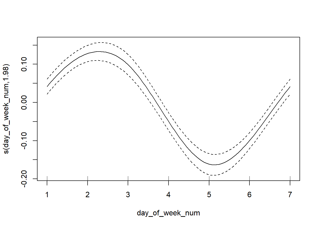
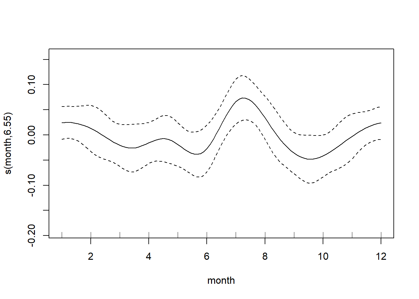
plot(generalized_additive_model, rug = T)

At this point, you’ll have to rely on your domain knowledge of the data. Here it seems reasonable to have a peak around Friday and Saturday and within the summer months. (Note: the data is overlapping with the tick marks, so the “rug” is a little hidden.)
What else can I do with GAMs?
If this post has you excited about GAMs, I give some more tips in my talk.
- Is your
gamcall taking too long? Try a “big” GAM:bam. - Want to smooth over two dimensions? Swap a smooth
s()for a tensor productte(). - Want to know if you need a curve or could just get away with a line? Take shrinkage for a spin and swap your
bs = "cr"forbs = "cs". - Want to buy back a little interpretability, try decomposing your
te()usingti()to see individual smooths and the leftover relationship between the two numerical covariates.
About the presenter
Sara Stoudt is a statistician with research interests in ecology and the communication of statistics. Sara received her bachelor’s degree in mathematics and statistics from Smith College and a doctorate in statistics from the University of California, Berkeley. Her graduate work involved evaluating species distribution and abundance models under model mis-specification. While at Berkeley she was also a Berkeley Institute for Data Science Fellow and worked with Professor Deborah Nolan to teach statistical writing. Keep an eye out for their forthcoming book, Communicating with Data: The Art of Writing for Data Science.
