The Basics

• Each user has a profile (page) and can add a photo and information about themselves
• Users can follow each other
• Users can tweet, i.e., publicly sharing a text/photo/link
• Each Tweet is restricted to a maximum of 280 characters
• Users can interact with a Tweet via comments (replies), likes, and shares (retweets)
• Users can interact with other users via direct messaging
• Users can create a thread: A series of connected tweets
• Users use hashtags (e.g., #mannheim) in order to associate their tweets with certain topics and to make them easier to find
• Users can search for keywords/hashtags in order to find relevant tweets and users

Twitter in Social Science Research

Analyzing tweets and social interaction on Twitter can help to answer social science research questions, especially in communication research and political science. Contrary to Facebook (API depreciation/shut-down in April 2018) and Instagram (API depreciation/shut-down in December 2018), Twitter data is (easily) accessible for researchers.

According to the Web of Science database, there are 2,598 journal articles published since 2009 with the word “Twitter” in their titles.

Figure 1: Number of articles by year

Figure 2: Number of articles by discipline

The Twitter API Platform

An API (Application Programming Interface) allows users to access (real-time) Twitter data. Twitter offers a variety of API services – some for free, others not. Using these services, one can search for tweets published in the past, stream tweets in realtime, and manage Twitter accounts and ads. The following exercises will focus on the free-of-charge API service, which is used in the vast majority of research projects: The Realtime Streaming API.

The Streaming API - Collecting Tweets in Realtime

“Establishing a connection to the streaming APIs means making a very long lived HTTP request, and parsing the response incrementally. Conceptually, you can think of it as downloading an infinitely long file over HTTP”. This way, we can receive up to a maximum of 1% of all tweets worldwide. As a query is usually specified by selected keywords or geographic areas, you will be able to collect (almost) all relevant tweets for your research interest. There are three filter parameters that you can use:

• ‘Follow’: Receive tweets of up to 5,000 users
• ‘Track’: Receive tweets that contain up to 400 keywords
• ‘Location’: Receive tweets from within a set of up to 25 geographic bounding boxes

API Authentification

You need to authenticate yourself when making requests to the Twitter API. Twitter uses the OAuth protocol, an “open protocol to allow secure authorization in a simple and standard method from web, mobile and desktop applications”. This involves five necessary steps:

• creating a Twitter account
• logging in to your Twitter account via https://developer.twitter.com/
• creating an app
• creating keys, access token & secret

Data Collection

There are a number of ways to collect Twitter data, including writing your own script to make continuous HTTP requests, Python’s tweepy package, and R’s rtweet package. The following demonstrates how to collect Twitter data using different Streaming API endpoints and the rtweet package.

Collecting Tweets Using the rtweet Package

As usual, we start with a little housekeeping: Installing required packages per install.packages() and specifying a working directory using setwd().

# Install Packages
install.packages("rtweet")
install.packages("ggmap")
install.packages("igraph")
install.packages("ggraph")
install.packages("tidytext")
install.packages("ggplot2")
install.packages("dplyr")
install.packages("readr")

# Set Working Directory
setwd("/PATH")

The code chunk below then illustrates three examples of collecting Twitter data using the rtweet package. After loading the required packages into the library(), we specify our authentication token per create_token() (see API Authentification above). After this, we are live: Using the function stream_tweets(), we collect:

1. a sample of current tweets for timeout = 10 seconds.
2. a sample of current tweets containing either of the keywords q = "trump, donald trump" for timeout = 30 seconds.
3. a sample of current tweets for timeout = 180 seconds from a specific location (in this instance, Berlin), restricting our search to a rectangular area defined by coordinates for longitude and latitude. Use, for instance, https://boundingbox.klokantech.com/ to retrieve the coordinates of your choosing.

# Open Libraries
library(rtweet)

# Speficy Authentification Token's provided in your Twitter App
create_token(
  app = "APPNAME",
  consumer_key = "consumer_key",
  consumer_secret = "consumer_secret",
  access_token = "access_token",
  access_secret = "access_secret"
)

# Collect a 'random' sample of Tweets for 10 seconds
stream_tweets(
  q = "",
  timeout = 10,
  file_name = "sample.json",
  parse = FALSE
)
sample <- parse_stream("sample.json")
save(sample, file = "sample_live.Rda")

# Collect Tweets that contain specific keywords for 30 seconds
stream_tweets(
  q = "trump, donald trump",
  timeout = 30,
  file_name = "trump.json",
  parse = FALSE
)
trump <- parse_stream("trump.json")
save(trump, file = "trump_live.Rda")

# Collect Tweets from a specific location
stream_tweets(
  c(13.0883,52.3383,13.7612,52.6755), 
  timeout = 180,
  file_name = "berlin.json",
  parse = FALSE
)
berlin <- parse_stream("berlin.json")
save(berlin, file = "berlin_live.Rda")

By running the steam_tweets() function, we receive Tweets and related meta-information from the Twitter API. The data is stored in .json format (Java Script Object Notation), though we can store these files as data frames after parsing them per parse_stream(). Each row in the data frame represents a Tweet or Re-Tweet and contains, amongst other, the following information:

• The content of a Tweet + Tweet-URL + Tweet-ID
• User-name + User-ID
• Time-stamp
• Place, country, geocodes (rarely)
• User self-description, residence, no. of followers, no. of friends
• URLs to images, videos

For illustration, we take the example of the data frame sample, the result of our first query. As we can see, our 10 second sample without specified key words contains 88 variables (columns) and 359 tweets (rows). You can see the full list of variables below, along with a small anonymized portion of five English language tweets (you can only see the first few characters of each tweet, stored in the variable sample$text).

# Dimensions of the data frame
dim(sample)

## [1] 359  88

# Variables in the data frame
names(sample)

##  [1] "user_id"                 "status_id"              
##  [3] "created_at"              "screen_name"            
##  [5] "text"                    "source"                 
##  [7] "display_text_width"      "reply_to_status_id"     
##  [9] "reply_to_user_id"        "reply_to_screen_name"   
## [11] "is_quote"                "is_retweet"             
## [13] "favorite_count"          "retweet_count"          
## [15] "hashtags"                "symbols"                
## [17] "urls_url"                "urls_t.co"              
## [19] "urls_expanded_url"       "media_url"              
## [21] "media_t.co"              "media_expanded_url"     
## [23] "media_type"              "ext_media_url"          
## [25] "ext_media_t.co"          "ext_media_expanded_url" 
## [27] "ext_media_type"          "mentions_user_id"       
## [29] "mentions_screen_name"    "lang"                   
## [31] "quoted_status_id"        "quoted_text"            
## [33] "quoted_created_at"       "quoted_source"          
## [35] "quoted_favorite_count"   "quoted_retweet_count"   
## [37] "quoted_user_id"          "quoted_screen_name"     
## [39] "quoted_name"             "quoted_followers_count" 
## [41] "quoted_friends_count"    "quoted_statuses_count"  
## [43] "quoted_location"         "quoted_description"     
## [45] "quoted_verified"         "retweet_status_id"      
## [47] "retweet_text"            "retweet_created_at"     
## [49] "retweet_source"          "retweet_favorite_count" 
## [51] "retweet_retweet_count"   "retweet_user_id"        
## [53] "retweet_screen_name"     "retweet_name"           
## [55] "retweet_followers_count" "retweet_friends_count"  
## [57] "retweet_statuses_count"  "retweet_location"       
## [59] "retweet_description"     "retweet_verified"       
## [61] "place_url"               "place_name"             
## [63] "place_full_name"         "place_type"             
## [65] "country"                 "country_code"           
## [67] "geo_coords"              "coords_coords"          
## [69] "bbox_coords"             "status_url"             
## [71] "name"                    "location"               
## [73] "description"             "url"                    
## [75] "protected"               "followers_count"        
## [77] "friends_count"           "listed_count"           
## [79] "statuses_count"          "favourites_count"       
## [81] "account_created_at"      "verified"               
## [83] "profile_url"             "profile_expanded_url"   
## [85] "account_lang"            "profile_banner_url"     
## [87] "profile_background_url"  "profile_image_url"

# An anonymized portion of the data frame, only tweets in English
sample$user_id <- seq(1, nrow(sample), 1)
sample$screen_name <- paste("name", seq(1, nrow(sample), 1), sep = "_")
sample <- subset(sample, lang == "en")
sample[1:5, c("user_id", "created_at", "screen_name", "text", "is_quote", 
              "is_retweet")]

## # A tibble: 5 x 6
##   user_id created_at          screen_name text          is_quote is_retweet
##     <dbl> <dttm>              <chr>       <chr>         <lgl>    <lgl>     
## 1       1 2019-04-03 10:22:32 name_1      just see..<U+2764><U+FE0F>~ FALSE    FALSE     
## 2       4 2019-04-03 10:22:33 name_4      I’m slowy gi~ FALSE    TRUE      
## 3      15 2019-04-03 10:22:33 name_15     "\"I didn't ~ TRUE     FALSE     
## 4      20 2019-04-03 10:22:33 name_20     Hmm. I’ma de~ FALSE    TRUE      
## 5      28 2019-04-03 10:22:33 name_28     I still hear~ TRUE     TRUE

Example 1: Prepping Tweets for Text Analysis

Quantitative Text Analysis (QTA) typically relies on pre-processed textual data (see this blog post for our SSDL workshop on QTA by Denise Traber). The code chunk below illustrates how a collection of Tweets can easily be prepared for QTA techniques such as content or sentiment analysis.

In this example, we use our 30 second sample of Tweets containing the key words “donald trump” and/or “trump”, which we stored as trump_live.RDa (see Collecting Tweets Using the rtweet Package above). Tweet contents are stored in the variable trump$text. Using the tidytextand dplyr packages, we then process the Tweets into a text corpus as follows:

1. Remove URLs from all tweets using gsub()
2. Remove punctuation, convert to lowercase, and seperate all words using unnest_tokens()
3. Remove stop words by first loading a list of stop words from the tidytext package via data("stop_words") and then removing these words from our tweets via anti_join(stop_words)

# Open Libraries
library(tidytext)
library(dplyr)

# Data Cleaning
# Delete Links in the Tweets
trump$text <- gsub("http.*", "", trump$text)
trump$text <- gsub("https.*", "", trump$text)
trump$text <- gsub("&amp;", "&", trump$text)

# Remove punctuation, convert to lowercase, seperate all words
trump_clean <- trump %>%
  dplyr::select(text) %>%
  unnest_tokens(word, text)

# Load list of stop words - from the tidytext package
data("stop_words")

# Remove stop words from your list of words
cleaned_tweet_words <- trump_clean %>%
  anti_join(stop_words)

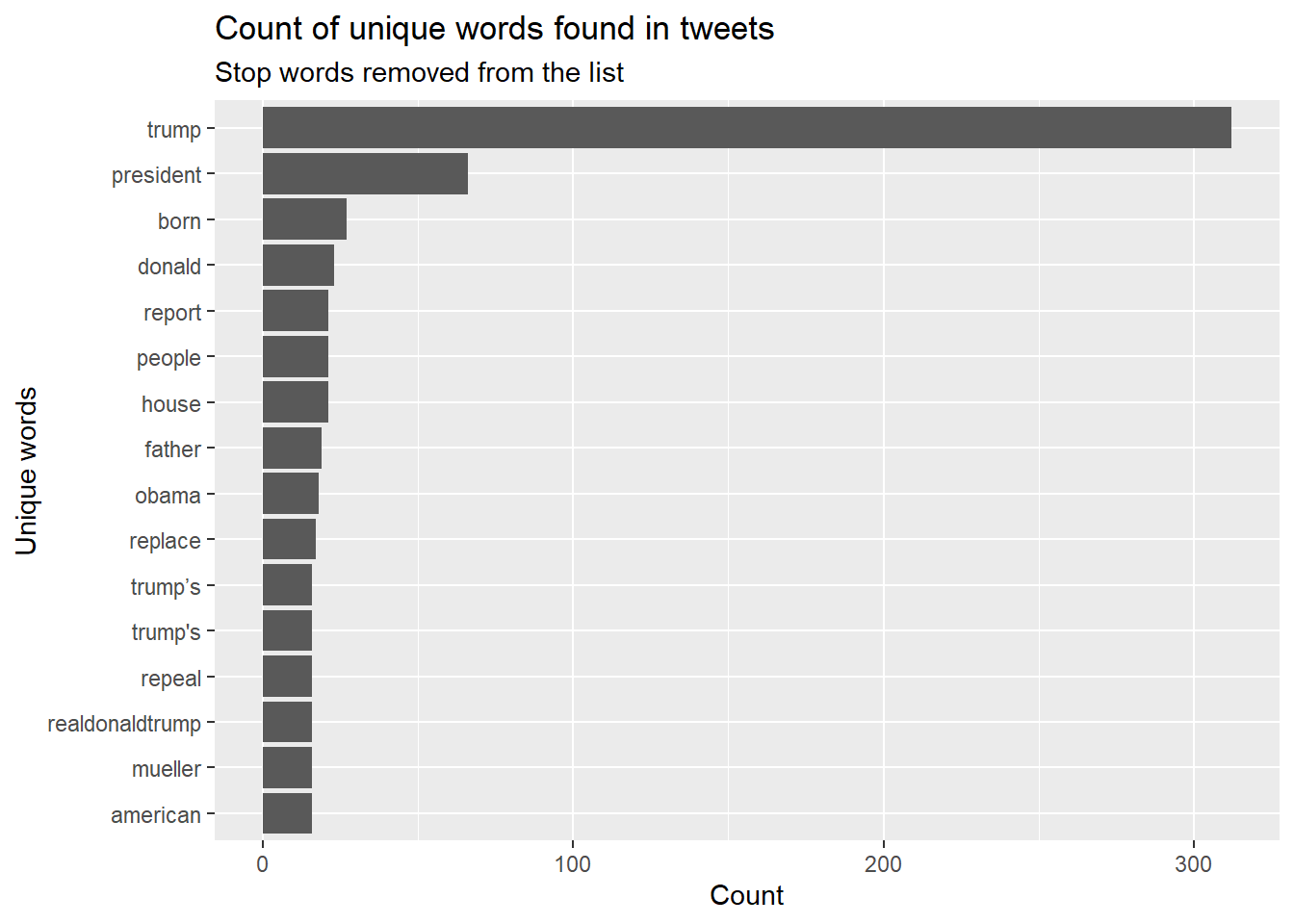
Following this, we can calculate the word counts in our Tweet collection and visualize the 15 most frequent words:

# Plot the top 15 words
cleaned_tweet_words %>%
  count(word, sort = TRUE) %>%
  top_n(15) %>%
  mutate(word = reorder(word, n)) %>%
  ggplot(aes(x = word, y = n)) +
  geom_col() +
  xlab(NULL) +
  coord_flip() +
  labs(y = "Count",
       x = "Unique words",
       title = "Count of unique words found in tweets",
       subtitle = "Stop words removed from the list")

## Selecting by n

Figure 3: Top 15 Most Frequent Words

Example 2: Analyzing Locations

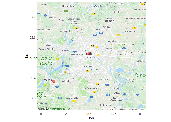
Provided that users share their exact geo-information, we can locate their tweets on geographical maps. For example, in our 3 minute sample of Tweets from berlin (see Collecting Tweets Using the rtweet Package above), this information was available for only two Tweets.

The code below demonstrates how one can view these Tweets mapped onto their exact geographical locations. We first pre-process the data, extracting numerical geo-coordinates for longitude and latitude where this information is available. We then subset the data frame to observations where these information exist. Lastly, using the same geo-coordinates as in the data collection, we set up an empty rectangular map of Berlin. Note that the last step involves accessing the Google Maps API, for which you will have to register separately (see, e.g., this post at R-bloggers).

library(ggmap)
library(dplyr)

# Seperate Geo-Information (Lat/Long) Into Two Variables
berlin <- tidyr::separate(data = berlin,
                          col = geo_coords,
                          into = c("Latitude", "Longitude"),
                          sep = ",",
                          remove = FALSE)

# Remove Parentheses
berlin$Latitude <- stringr::str_replace_all(berlin$Latitude, "[c(]", "")
berlin$Longitude <- stringr::str_replace_all(berlin$Longitude, "[)]", "")

# Store as numeric
berlin$Latitude <- as.numeric(berlin$Latitude)
berlin$Longitude <- as.numeric(berlin$Longitude)

# Keep only those tweets where geo information is available
berlin <- subset(berlin, !is.na(Latitude) & !is.na(Longitude))

# Set up empty map
berlin_map <- get_map(location = c(lon = mean(c(13.0883, 13.7612)),
                                   lat = mean(c(52.3383, 52.6755))),
                      zoom = 10,
                      maptype = "terrain",
                      source = "google")

Building up on this, we can then map our collected tweets to see from where they were sent: Berlin-Mitte and Potsdam.

tweet_map <- ggmap(berlin_map)
tweet_map + geom_point(data = berlin,
                       aes(x = Longitude,
                           y = Latitude),
                           color = "red",
                           size = 4,
                           alpha = .5)

Figure 4: GPS Coordinates of 2 Tweets

Bias and Representativity

Twitter users do not represent a random sample from a given population. This is not only due to the presence of bots and company or institutional accounts, but also to the manifold self-selection processes that using Twitter entails:

Population → Internet Users → Twitter Users → Active Twitter Users → Users sharing geo-information

Below are some references that analyze the magnitude and severity of these (and related) problems:

• Barberá, P. & G. Rivero, 2015: Understanding the Political Representativeness of Twitter Users. Social Science Computer Review 33(6) 712-729.
• Mellon, J. & C. Prosser, 2017: Twitter and Facebook are not representative of the general population: Political attitudes and demographics of British social media users. Research and Politics 2017: 1-9.
• Hölig, S., 2018: Eine meinungsstarke Minderheit als Stimmungsbarometer?! Über die Persönlichkeitseigenschaften aktiver Twitterer. M&K Medien- und Kommunikationswissenschaft 66: 140-169.

Replicability and Black-Box Twitter

Real-time Twitter data collection is not reproducible and for a given query. Furthermore, you can only hope that Twitter will provide you with a true random sample of Tweets. If completeness is crucial for your research interest, you will have to pay for complete access to all Tweets ever tweeted: “Both Historical PowerTrack and Full-Archive Search provide access to any publicly available Tweet, starting with the first Tweet from March 2006”.

Data Privacy and Research Ethics

Tweets on public Twitter profiles are generally available. There are no measures in place that prevent the collection and analysis of the data, and users’ consent for the collection and processing of their tweets and profile information is usually not required. This practice is also congruous with certain guidelines for academic and commerical social media research (e.g DGOF Richtlinien zur Social Media Forschung: “In offenen Sozialen Medien bzw. den entsprechenden Bereichen dürfen die personenbezogenen Daten der Teilnehmer grundsätzlich ohne entsprechende explizite Einwilligung auf der Grundlage der gesetzlichen Erlaubnisnorm auch für Zwecke der Markt- und Sozialforschung verarbeitet und genutzt werden.”

However, Twitter’s terms of service are not necessarily congruous with German or EU data protection regulations (e.g. DSGVO). Ultimately, this leaves the ethical and legal questions of how to ensure data privacy to us as researchers. Should we, for instance, further anonymize data, e.g. by separating user IDs from Tweet content and meta-information? What are the implications for open science? Should the full data, including user IDs and geo locations be publicly and permanently shared (e.g., as part of replication materials)? Should the answer to these questions be the same for regular users as opposed to public figures (e.g., politicians)? These questions highlight the urgent need for ongoing discussion about these topics.

Uncertainty of Data Access

One should always have in mind that data access is 100% dependent upon Twitter’s willingness to share the data, and therby also on jurisdiction by which Twitter must abide (think, for instance, about Article 13). Data access for research projects through Facebook’s and Instagram’s APIs has previously been shut-down completely with only few weeks notice. Given that, research projects relying on Twitter data are always risky. This applies particularly to research projects that depends on a constant Twitter data influx over a long period of time (e.g., PhD projects).

Data Storage

Data storage can be an issue when tweets are collected over a long period of time. In many applications, data collections can easily amount to 100-200 GB per month. The use of powerful servers and storage in a relational database (e.g. SQL) are therefore recommended.