Advancing Text Mining with R and quanteda
Everyone is talking about text analysis. Is it puzzling that this data source is so popular right now? Actually no. Most of our datasets rely on (hand-coded) textual information. Extracting, processing, and analyzing this oasis of information becomes increasingly relevant for a large variety of research fields. This Methods Bites Tutorial by Cosima Meyer summarizes Cornelius Puschmann’s workshop in the MZES Social Science Data Lab in January 2019 on advancing text mining with R and the package quanteda. The workshop offered guidance through the use of quanteda and covered various classification methods, including classification with known categories (dictionaries and supervised machine learning) and with unknown categories (unsupervised machine learning).
This post was updated in December 2020 to be consistent with quanteda’s version 2.1.2. For more information on differences between quanteda versions, have a look at this excellent overview.
Overview
This blog post is based on this report and on Cornelius’ post on topic models in R.
What is quanteda?
In order to analyze text data, R has several packages available. In this blog post we focus on quanteda. quanteda is one of the most popular R packages for the quantitative analysis of textual data that is fully-featured and allows the user to easily perform natural language processing tasks. It was originally developed by Ken Benoit and other contributors. It offers an extensive documentation and is regularly updated. quanteda is most useful for preparing data that can then be further analyzed using unsupervised/supervised machine learning or other techniques. A combination with tidyverse leads to a more transparent code structure and offers a mere variety of useful areas that could not be addressed within the limited time of the workshop (e.g., scaling models, part-of-speech (POS) tagging, named entities, word embeddings, etc.).
There are also similar R packages such as tm, tidytext, and koRpus. tm has simpler grammer but slightly fewer features, tidytext is very closely integrated with dplyr and well-documented, and koRpus is good for tasks such as part-of-speech (POS) tagging).
How do we use quanteda?
Most analyses in quanteda require three steps:
1. Import the data
The data that we usually use for text analysis is available in text formats (e.g., .txt or .csv files).
2. Build a corpus
After reading in the data, we need to generate a corpus. A corpus is a type of dataset that is used in text analysis. It contains “a collection of text or speech material that has been brought together according to a certain set of predetermined criteria” (Shmelova et al. 2019, p. 33). These criteria are usually set by the researchers and are in concordance with the guiding question. For instance, if you are interested in analyzing speeches in the UN General Debate, these predetermined criteria are the time and scope conditions of these debates (speeches by countries at different points in time).
3. Calculate a document-feature matrix (DFM)
Another essential component for text analysis is a document-feature matrix (DFM); also called document-term matrix (DTM). These two terms are synonyms but quanteda refers to a DFM whereas others will refer to DTM. It describes how frequently terms occur in the corpus by counting single terms.
To generate a DFM, we first split the text into its single terms (tokens). We then count how frequently each term (token) occurs in each document.
The following graphic describes visually how we turn raw text into a vector-space representation that is easily accessible and analyzable with quantitative statistical tools. It also visualizes how we can think of a DFM. The rows represent the documents that are part of the corpus and the columns show the different terms (tokens). The values in the cells indicate how frequently these terms (tokens) are used across the documents.
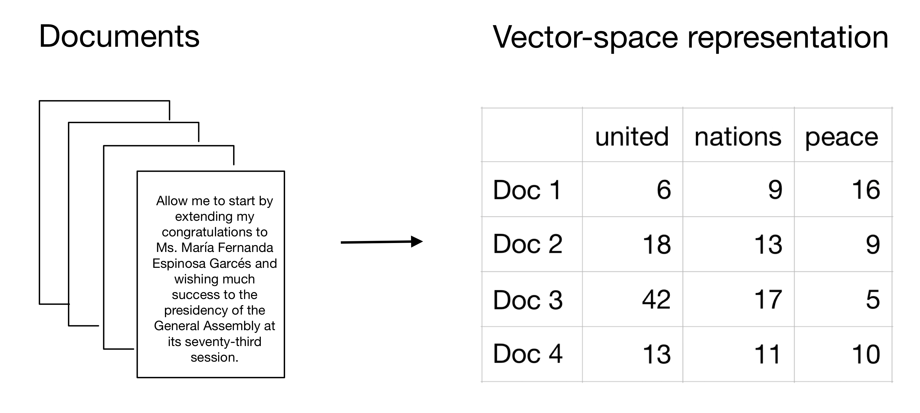
Figure 1: Model of a DFM
Important things to remember about DFMs:
- A corpus is positional (string of words) and a DFM is non-positional (bag of words). Put differently, the order of the words matters in a corpus whereas a DFM does not have information on the position of words.
- A token is each individual word in a text (but it could also be a sentence, paragraph, or character). This is why we call creating a “bag of words” also tokenizing text. In a nutshell, a DFM is a very efficient way of organizing the frequency of features/tokens but does not contain any information on their position. In our example, the features of a text are represented by the columns of a DFM and aggregate the frequency of each token.
- In most projects you want one corpus to contain all your data and generate many DFMs from that.
- The rows of a DFM can contain any unit on which you can aggregate documents. In the example above, we used the single documents as the unit. It may also well be more fine-grained with sub-documents or more aggregated with a larger collection of documents.
- The columns of a DFM are any unit on which you can aggregate features. Features are extracted from the texts and quantitatively measurable. Features can be words, parts of the text, content categories, word counts, etc. In the example above, we used single words such as “united”, “nations”, and “peace”.
To showcase the three steps introduced above, we are using the UN General Debate data by Mikhaylov, Baturo, and Dasandi dataset. There is also a pre-processed version of the dataset accessible with quanteda.corpora.
How to access the UNGD data with
quanteda.corpora
# Install package quanteda.corpora
devtools::install_github("quanteda/quanteda.corpora")

# Load the dataset
quanteda.corpora::data_corpus_ungd2017
We will, however, mainly rely on the original dataset throughout the following explanations to match closely the regular workflow of textual data in R. If you want to replicate the steps, please download the data here and unzip the zip file. Your global_path should direct you to the text file folders.
In a first step, we need to load the necessary packages and read in the data.
# Load all required packages
library(tidyverse)        # Also loads dplyr, ggplot2, and haven
library(quanteda)         # For NLP
library(readtext)         # To read .txt files
library(stm)              # For structural topic models
library(stminsights)      # For visual exploration of STM
library(wordcloud)        # To generate wordclouds
library(gsl)              # Required for the topicmodels package
library(topicmodels)      # For topicmodels
library(caret)            # For machine learning

# Download data here:
# https://dataverse.harvard.edu/dataset.xhtml?persistentId=doi:10.7910/DVN/0TJX8Y
# and unzip the zip file

# Read in data (.txt files)
global_path <- "path/to/folder/UN-data/"

# We load the data (.txt files) from all subfolders (readtext can handle
# this without specification)  and store them in the main UNGDspeeches
# dataframe. Beyond the speech text, this data also includes the
# meta-data from the text filenames and add variables for the country,
# UN session, and year.
# The code is based on https://github.com/quanteda/quanteda.corpora/issues/6
# and https://github.com/sjankin/UnitedNations/blob/master/files/UNGD_analysis_example.Rmd

# For the purpose of this blog post, we use the data from all sessions.
UNGDspeeches <- readtext(
  paste0(global_path, "*/*.txt"),
  docvarsfrom = "filenames",
  docvarnames = c("country", "session", "year"),
  dvsep = "_",
  encoding = "UTF-8"
)
We can then proceed and generate a corpus.
mycorpus <- corpus(UNGDspeeches)

# Assigns a unique identifier to each text
docvars(mycorpus, "Textno") <-
  sprintf("%02d", 1:ndoc(mycorpus))
As we can see (by calling the object mycorpus), the corpus consists of 8,093 documents.
Output:
mycorpus
mycorpusCorpus consisting of 8,093 documents and 4 docvars.With this data, we can already generate first descriptive statistics.
# Save statistics in "mycorpus.stats"
mycorpus.stats <- summary(mycorpus)

# And print the statistics of the first 10 observations
head(mycorpus.stats, n = 10)
# Text Types Tokens Sentences country session year Textno
# 1 ALB_25_1970.txt 1727 9077 256 ALB 25 1970 01
# 2 ARG_25_1970.txt 1425 5192 218 ARG 25 1970 02
# 3 AUS_25_1970.txt 1611 5688 270 AUS 25 1970 03
# 4 AUT_25_1970.txt 1340 4717 164 AUT 25 1970 04
# 5 BEL_25_1970.txt 1289 4783 207 BEL 25 1970 05
# 6 BLR_25_1970.txt 1427 6138 204 BLR 25 1970 06
# 7 BOL_25_1970.txt 1559 5612 225 BOL 25 1970 07
# 8 BRA_25_1970.txt 1333 4422 154 BRA 25 1970 08
# 9 CAN_25_1970.txt 728 1887 97 CAN 25 1970 09
# 10 CMR_25_1970.txt 928 3144 106 CMR 25 1970 10In a next step, we can also calculate the document-feature matrix. To do so, first we need to generate tokens (tokens()) and can also already pre-process the data. This includes removing the numbers (remove_numbers), punctuations (remove_punct), symbols (remove_symbols), and urls beginning with http(s) (remove_url).
An earlier version of this blog post used remove_hyphens to remove hyphens as well as remove_twitterto remove symbols such as @ and #. Both commands are either deprecated or defunctional. To remove hyphens, it is recommended to use split_hyphens instead. For twitter symbols there is no new command. Quanteda’s manual recommends to use ``an alternative tokenizer, including non-quanteda options’’.
We further include the docvars from our corpus (include_docvars).
# Preprocess the text

# Create tokens
token <-
  tokens(
    mycorpus,
    split_hyphens = TRUE,
    remove_numbers = TRUE,
    remove_punct = TRUE,
    remove_symbols = TRUE,
    remove_url = TRUE,
    include_docvars = TRUE
  )
Since the pre-1994 documents were scanned with OCR scanners, several tokens with combinations of digits and characters were introduced. We clean them manually following this guideline.
# Clean tokens created by OCR
token_ungd <- tokens_select(
  token,
  c("[\\d-]", "[[:punct:]]", "^.{1,2}$"),
  selection = "remove",
  valuetype = "regex",
  verbose = TRUE
)
In the next step, we then create the document-feature matrix. We lower and stem the words (tolower and stem) and remove common stop words (remove=stopwords()). Stopwords are words that appear in texts but do not give the text a substantial meaning (e.g., “the”, “a”, or “for”). Since the language of all documents is English, we only remove English stopwords here. quanteda can also deal with stopwords from other languages (for more information see here).
mydfm <- dfm(token_ungd,
             tolower = TRUE,
             stem = TRUE,
             remove = stopwords("english")
             )
We can also trim the text with dfm_trim. Using the command and its respective specifications, we filter words that appear less than 7.5% and more than 90%. This rather conservative approach is possible because we have a sufficiently large corpus.
mydfm.trim <-
  dfm_trim(
    mydfm,
    min_docfreq = 0.075,
    # min 7.5%
    max_docfreq = 0.90,
    #  max 90%
    docfreq_type = "prop"
  )
To get a look at the DFM, we now print their first 5 observations and first 10 features:
# And print the results of the first 10 observations and first 10 features in a DFM
head(dfm_sort(mydfm.trim, decreasing = TRUE, margin = "both"),
     n = 10,
     nf = 10)
Document-feature matrix of: 5 documents, 10 features (4.0% sparse) and 4 docvars.
features
docs problem session conflict council africa global resolut hope south situat
CUB_34_1979.txt 36 8 1 0 13 3 10 8 10 23
IRL_39_1984.txt 41 9 18 11 14 5 16 21 19 9
PAN_37_1982.txt 14 12 12 8 11 2 6 11 20 10
BFA_29_1974.txt 25 17 1 4 15 0 10 20 6 9
GRC_43_1988.txt 27 9 13 14 10 2 10 10 11 5The sparsity gives us information about the proportion of cells that have zero counts.
Classification
A next step can involve the classification of the text. The article by Grimmer and Stewart (2013) provides a good overview for this step. The upcoming section follows their structure. Classification sorts texts into categories. The following picture is leaned on the figure by Grimmer and Stewart (2013, 268) and illustrates a possible structure of classification.
)](/../../../../article/advancing-text-mining/figures/overview.png)
Figure 2: Overview of classification (own illustration, based on Grimmer and Stewart (2013, 268))
A researcher usually faces one of the following situations: The categories are known beforehand or the categories are unknown. If the researcher knows the categories, s/he can use automated methods to minimize the workload that is associated with the categorization of the texts. Throughout the workshop, two methods were presented: a dictionary method and a supervised method. If the researcher does not know the categories, s/he is likely to resort to unsupervised machine learning. The following section provides illustrative examples for both methods.
Known categories
Known categories: Dictionaries
Dictionaries contain lists of words that correspond to different categories. If we apply a dictionary approach, we count how often words that are associated with different categories are represented in each document. These dictionaries help us to classify (or categorize) the speeches based on the frequency of the words that they contain. Popular dictionaries are sentiment dictionaries (such as Bing, Afinn or LIWC) or LexiCoder.
We use the “LexiCoder Policy Agenda” dictionary that can be accessed here in a .lcd format. The “LexiCoder Policy Agenda” dictionary captures major topics from the comparative Policy Agenda project and is currently available in Dutch and English.
To read in the dictionary, we use quanteda’s built-in function dictionary().
# load the dictionary with quanteda's built-in function
dict <- dictionary(file = "policy_agendas_english.lcd")
We apply this dictionary to filter the share of each country’s speeches on immigration, international affair and defence.
mydfm.un <- dfm(mydfm.trim, groups = "country", dictionary = dict)

un.topics.pa <- convert(mydfm.un, "data.frame") %>%
  dplyr::rename(country = doc_id) %>%
  select(country, immigration, intl_affairs, defence) %>%
  tidyr::gather(immigration:defence, key = "Topic", value = "Share") %>%
  group_by(country) %>%
  mutate(Share = Share / sum(Share)) %>%
  mutate(Topic = haven::as_factor(Topic))
In a next step, we can visualize the results with ggplot. This gives us a first impression of the distribution of the topics in the 2018 UN General Debate across countries.
un.topics.pa %>%
  ggplot(aes(country, Share, colour = Topic, fill = Topic)) +
  geom_bar(stat = "identity") +
  scale_colour_brewer(palette = "Set1") +
  scale_fill_brewer(palette = "Pastel1") +
  ggtitle("Distribution of PA topics in the UN General Debate corpus") +
  xlab("") +
  ylab("Topic share (%)") +
  theme(axis.text.x = element_blank(),
        axis.ticks.x = element_blank())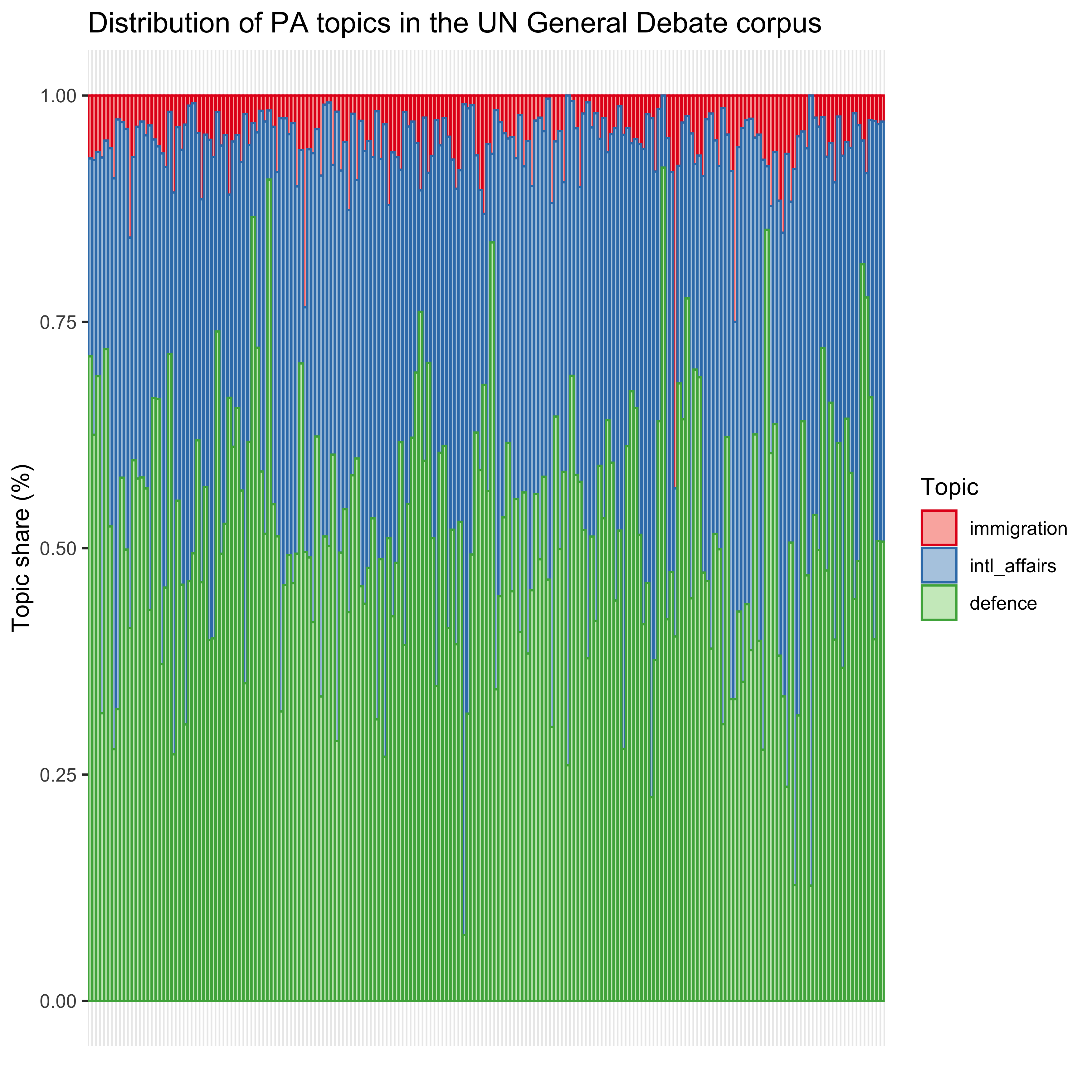
Figure 3: Distribution of PA topics in the UN General Debate corpus
We observe a relatively high share for both defence and international affairs whereas immigration receives fewer attention in the speeches.
Known categories: Supervised machine learning - Naive Bayes (NB)
We now turn to supervised machine learning. Similar to the dictionary approach explained above, this method also requires some pre-existing classifications. But in contrast to a dictionary, we now divide the data into a training and a test dataset. This follows the general logic of machine learning algorithms. The training data already contains the classifications and trains the algorithm (e.g., our Naive Bayes classifier) to predict the class of our speech based on the features that are given. A Naive Bayes classifier now calculates the probability for each class based on the features. It eventually goes for the class with the highest probability and selects this class as the corresponding category. It is based on the Bayes theorem for conditional probability. It can be formally written as: \[ P(A | B) = \frac{P(A) * P(B | A)}{P(B)}\] In plain words, the probability of A is conditional on B.
Bayes’ theorem
- \(A\) and \(B\) are events
- \(P(A)\) and \(P(B)\) is the probability of observing \(A\) and \(B\) (respectively) independent from each other
- \(P(A) \neq 0\) and \(P(B) \neq 0\)
- \(P(A|B)\) is the conditional probability that \(A\) occurs when \(B\) is true \[P(A|B) = \frac{P(A \cap B)}{P(B)}, if P(B) \neq 0\]
- \(P(B|A)\) is the conditional probability that \(B\) occurs when \(A\) is true \[P(B|A) = \frac{P(B \cap A)}{P(A)}, if P(A) \neq 0\]
- And we also have the joint probability of $ P(A B) = P(B A)$ because
Why is Naive Bayes “naive”? Naive Bayes is “naive” because of its strong independence assumptions. It assumes that all features are equally important and that all features are independent. If you think of n-grams and compare unigrams and bigrams, you can intuitively understand why the last assumption is a strong assumption. A unigram counts each word as a gram (“I” “like” “walking” “in” “the” “sun”) whereas a bigram counts two words as a gram (“I like” “like walking” “walking in” “in the” “the sun”).
However, even when the assumptions are not fully met, Naive Bayes still performs well.
A Naive Bayes is a relatively simple classification algorithm because it does not require much time and working capacity of your machine. To use a Naive Bayes classifier, we rely on quanteda’s built-in function textmodel_nb.
To perform the Naive Bayes estimation, we proceed with the following steps:
1. We set up training and test data based on the corpus. 2. Based on these two datasets, we generate a DFM. 3. We train the algorithm by feeding in the training data and eventually use the test data for performance. 4. We then check the performance (accuracy) of our results. 5. And compare it with a random prediction.
For this example, we use the pre-labeled dataset that is used for the algorithm newsmap by Kohei Watanabe. The dataset contains information on the geographical location of newspaper articles. We introduce this new dataset as Naive Bayes – a supervised machine learning algorithm – requires pre-labeled data.
We first load the dataset. To do so, we follow Kohei Watanabe’s description here, download the corpus of Yahoo News from 2014, and follow the subsequent processing steps he describes.
# load data
load("../newspaper.RData")

# transform variables
pred_data$text <- as.character(pred_data$text)
pred_data$country <- as.character(pred_data$country)
For simplicity, we keep only the USA, Great Britain, France, Brazil, and Japan.
pred_data <- pred_data %>%
  dplyr::filter(country %in% c("us", "gb", "fr", "br", "jp")) %>%
dplyr::select(text, country)head(pred_data)| row | text | country |
|---|---|---|
| 1 | ’08 French champ Ivanovic loses to Safarova in 3rd. PARIS (AP) - Former French Open champion Ana Ivanovic lost in the third round Saturday, beaten 6-3, 6-3 by 23rd-seeded Lucie Safarova of the Czech Republic. | fr |
| 2 | Up to USD1,000 a day to care for child migrants. More than 57,000 unaccompanied children, mostly from Central America, have been caught entering the country illegally since last October, and President Barack Obama has asked for USD3.7 billion in emergency funding to address what he has called an ‘urgent humanitarian solution.’ ‘One of the figures that sticks in everybody’s mind is we’re paying about USD250 to USD1,000 per child,’ Senator Jeff Flake told reporters, citing figures presented at a closed-door briefing by Homeland Security Secretary Jeh Johnson. Federal authorities are struggling to find more cost-effective housing, medical care, counseling and legal services for the undocumented minors. The base cost per bed was USD250 per day, including other services, Senator Dianne Feinstein said, without providing details. | us |
| 3 | 1,400 gay weddings in England, Wales in first three months. Just over 1,400 gay couples tied the knot in the three months after same-sex marriage was allowed in England and Wales, figures out Thursday showed. The Office for National Statistics said 1,409 marriages took place between March 29 and June 30. ‘The novelty and significance of marriage becoming available led to an initial rush among same-sex couples wanting to be among the very first to assume the same rights and protection afforded to heterosexual couples,’ said James Brown, a partner at law firm JMW Solicitors. The figures will likely surge from December once civil partnerships can be converted into marriages. | gb |
| 4 | 1 dead after fan fighting in Brazil. SAO PAULO (AP) - Police say a 21-year-old man died after a confrontation between rival football fan groups in Brazil on Sunday. | br |
| 5 | 1 dead as plane with French tourists crashes in US. PAGE, Arizona (AP) - Authorities say a small plane carrying French tourists crashed while trying to land at an airport in Arizona, and one person was killed and another hospitalized. | fr |
| 6 | 1 US theory is someone diverted missing plane. WASHINGTON (AP) - A U.S. official says investigators are examining the possibility that someone caused the disappearance of a Malaysia Airlines jet with 239 people on board, and that it may have been ‘an act of piracy.’ | us |
We pre-process the data again. Our final corpus thus includes the newspaper headlines by country.
data_corpus <- corpus(pred_data, text_field = "text")In a first step, we need to define our training and our test dataset. Based on these two datasets, we generate a DFM. This code is based on Cornelius code and quanteda’s example. To do so, we apply similar general data pre-processing steps as discussed above.
# Set a seed for replication purposes
set.seed(68159)

# Generate random 10,000 numbers without replacement
training_id <- sample(1:29542, 10000, replace = FALSE)

# Create docvar with ID
docvars(data_corpus, "id_numeric") <- 1:ndoc(data_corpus)

# Get training set
dfmat_training <-
  corpus_subset(data_corpus, id_numeric %in% training_id) %>%
  dfm(stem = TRUE)

# Get test set (documents not in training_id)
dfmat_test <-
  corpus_subset(data_corpus,!id_numeric %in% training_id) %>%
  dfm(stem = TRUE)
We can now check the distribution of the countries across the two DFMs:
print(prop.table(table(docvars(
  dfmat_training, "country"
))) * 100)
br fr gb jp us
13.34 14.37 33.65 11.10 27.54 print(prop.table(table(docvars(
dfmat_test, "country"
))) * 100) br fr gb jp us
13.70893 15.13151 33.02630 10.93542 27.19783 As we can see, the countries are equally distributed across both DFMs.
In a next step, we train the Naive Bayes classifier. Going back to the formula stated above, we know that A is conditional on B.
\[ P(A | B) = \frac{P(A) * P(B | A)}{P(B)}\]
A is what we want to know (the country that is mainly addressed in each text) and B is what we see (the text). We can now proceed and replace A and B with the respective terms. This leads us to the next equation:
\[ P(Country | Text) = \frac{P(Country) * P(Text | Country)}{P(Text)}\]
We can then proceed and train our algorithm using quanteda’s built-in function textmodel_nb.
# Train naive Bayes
# The function takes a DFM as the first argument
model.NB <-
  textmodel_nb(dfmat_training, docvars(dfmat_training, "country"), prior = "docfreq")

# The prior indicates an assumed distribution.
# Here we choose how frequently the categories occur in our data.
dfmat_matched <-
dfm_match(dfmat_test, features = featnames(dfmat_training))The command summary(model.NB) gives us the results of our prediction. Click unfold to see the results.
Code:
summary(model.NB)
summary(model.NB)Call:
textmodel_nb.dfm(x = dfmat_training, y = docvars(dfmat_training,
"country"), prior = "docfreq")
Class Priors:
(showing first 5 elements)
br fr gb jp us
0.1334 0.1437 0.3365 0.1110 0.2754
Estimated Feature Scores:
' 08 french champ ivanov lose to safarova in 3rd . pari
br 0.08949 0.1679 0.007791 0.07636 0.08195 0.08707 0.09989 0.1474 0.1214 0.34322 0.1176 0.008863
fr 0.14212 0.2778 0.940061 0.37912 0.20345 0.16469 0.13803 0.3659 0.1473 0.24345 0.1296 0.947706
gb 0.43332 0.1532 0.032008 0.24397 0.14963 0.49395 0.35845 0.1346 0.3540 0.17905 0.3321 0.032363
jp 0.06507 0.1184 0.004396 0.10771 0.28900 0.06580 0.10287 0.1040 0.1007 0.06916 0.1059 0.002778
us 0.27000 0.2827 0.015743 0.19285 0.27598 0.18850 0.30077 0.2482 0.2766 0.16512 0.3148 0.008290
( ap ) - former open champion ana lost the third round
br 0.16080 0.24091 0.16100 0.1611 0.09034 0.17116 0.12708 0.08142 0.08045 0.1101 0.08964 0.30833
fr 0.14221 0.14820 0.14219 0.1363 0.17312 0.18636 0.24110 0.13475 0.16643 0.1350 0.17178 0.19535
gb 0.34860 0.28303 0.34870 0.3403 0.45720 0.36654 0.51497 0.07433 0.38923 0.3603 0.39194 0.24189
jp 0.09123 0.08125 0.09126 0.0922 0.04583 0.07443 0.05684 0.22969 0.07943 0.1005 0.07653 0.04757
us 0.25715 0.24661 0.25685 0.2702 0.23351 0.20152 0.06002 0.47982 0.28446 0.2940 0.27010 0.20686
saturday , beaten 6-3 by 23rd-seed
br 0.14287 0.1078 0.19323 0.21226 0.09731 0.1955
fr 0.19921 0.1384 0.20558 0.40985 0.12900 0.3236
gb 0.44845 0.3437 0.45359 0.21530 0.33256 0.1785
jp 0.09248 0.1099 0.07787 0.08317 0.11636 0.1379
us 0.11699 0.3001 0.06972 0.07942 0.32477 0.1646To better understand how well we did, we can also generate two frequency tables for right and wrong predictions.
prop.table(table(predict(model.NB) == docvars(dfmat_training, "country"))) * 100FALSE TRUE
2.71 97.29 To check if this result indicates a good performance, we compare it with a random result. We randomize the list of countries (and keep the overall frequency distribution of our countries constant) to allow our random algorithm a legitimate chance for a correct classification.
prop.table(table(sample(predict(model.NB)) == docvars(dfmat_training, "country"))) * 100FALSE TRUE
76.63 23.37 As we can see from the the summarized table below, our Naive Bayes classifier clearly outperforms a random algorithm.
| Naive Bayes | Random | |
|---|---|---|
| False | 2.71 | 76.63 |
| True | 97.29 | 23.37 |
We are likely to increase our accuracy even more by pre-processing our text data.
A confusion matrix helps us assess how well our algorithm performed. It shows us the prediction for all five countries in contrast to the actual class that is given by our data. For example, we predict 2580 articles as belonging to Great Britain that actually belong to Great Britain. However, we also predict 39 articles as British articles while they are actually French. Overall, when we look at the diagonal, we see that most predictions correctly classify the articles and that our algorithm performs well.
actual_class <- docvars(dfmat_matched, "country")
predicted_class <- predict(model.NB, newdata = dfmat_matched)
tab_class <- table(actual_class, predicted_class)
tab_class
predicted_class
actual_class br fr gb jp us
br 2580 6 50 6 37
fr 39 2697 124 11 86
gb 24 52 6072 24 282
jp 33 9 31 1945 119
us 56 32 194 66 4967We store our confusion matrix in an object because we need it later to visualize the results.
confusion <- confusionMatrix(tab_class, mode = "everything")Confusion Matrix and Statistics
             predicted_class
actual_class   br   fr   gb   jp   us
          br 2580    6   50    6   37
          fr   39 2697  124   11   86
          gb   24   52 6072   24  282
          jp   33    9   31 1945  119
          us   56   32  194   66 4967
Overall Statistics
Accuracy : 0.9344
95% CI : (0.9309, 0.9379)
No Information Rate : 0.3311
P-Value [Acc > NIR] : < 2.2e-16
Kappa : 0.914
Mcnemar's Test P-Value : < 2.2e-16
Statistics by Class:
Class: br Class: fr Class: gb Class: jp Class: us
Sensitivity 0.9444 0.9646 0.9383 0.94786 0.9046
Specificity 0.9941 0.9845 0.9708 0.98902 0.9752
Pos Pred Value 0.9630 0.9121 0.9408 0.91015 0.9345
Neg Pred Value 0.9910 0.9940 0.9695 0.99385 0.9632
Precision 0.9630 0.9121 0.9408 0.91015 0.9345
Recall 0.9444 0.9646 0.9383 0.94786 0.9046
F1 0.9536 0.9376 0.9396 0.92862 0.9193
Prevalence 0.1398 0.1431 0.3311 0.10500 0.2810
Detection Rate 0.1320 0.1380 0.3107 0.09953 0.2542
Detection Prevalence 0.1371 0.1513 0.3303 0.10935 0.2720
Balanced Accuracy 0.9692 0.9745 0.9546 0.96844 0.9399To display our confusion matrix visually, we could either produce a heatmap or a confusion matrix.
We first plot a heatmap using the code below.
Code: Heatmap using
ggplot2
# Save confusion matrix as data frame
confusion.data <- as.data.frame(confusion[["table"]])

# Reverse the order
level_order_y <-
  factor(confusion.data$actual_class,
         level = c('us', 'jp', 'gb', 'fr', 'br'))

ggplot(confusion.data,
       aes(x = predicted_class, y = level_order_y, fill = Freq)) +
  xlab("Predicted class") +
  ylab("Actual class") +
  geom_tile() + theme_bw() + coord_equal() +
  scale_fill_distiller(palette = "Blues", direction = 1) +
  scale_x_discrete(labels = c("Brazil", "France", "Great \n Britain", "Japan", "USA")) +
  scale_y_discrete(labels = c("USA", "Japan", "Great \n Britain", "France", "Brazil"))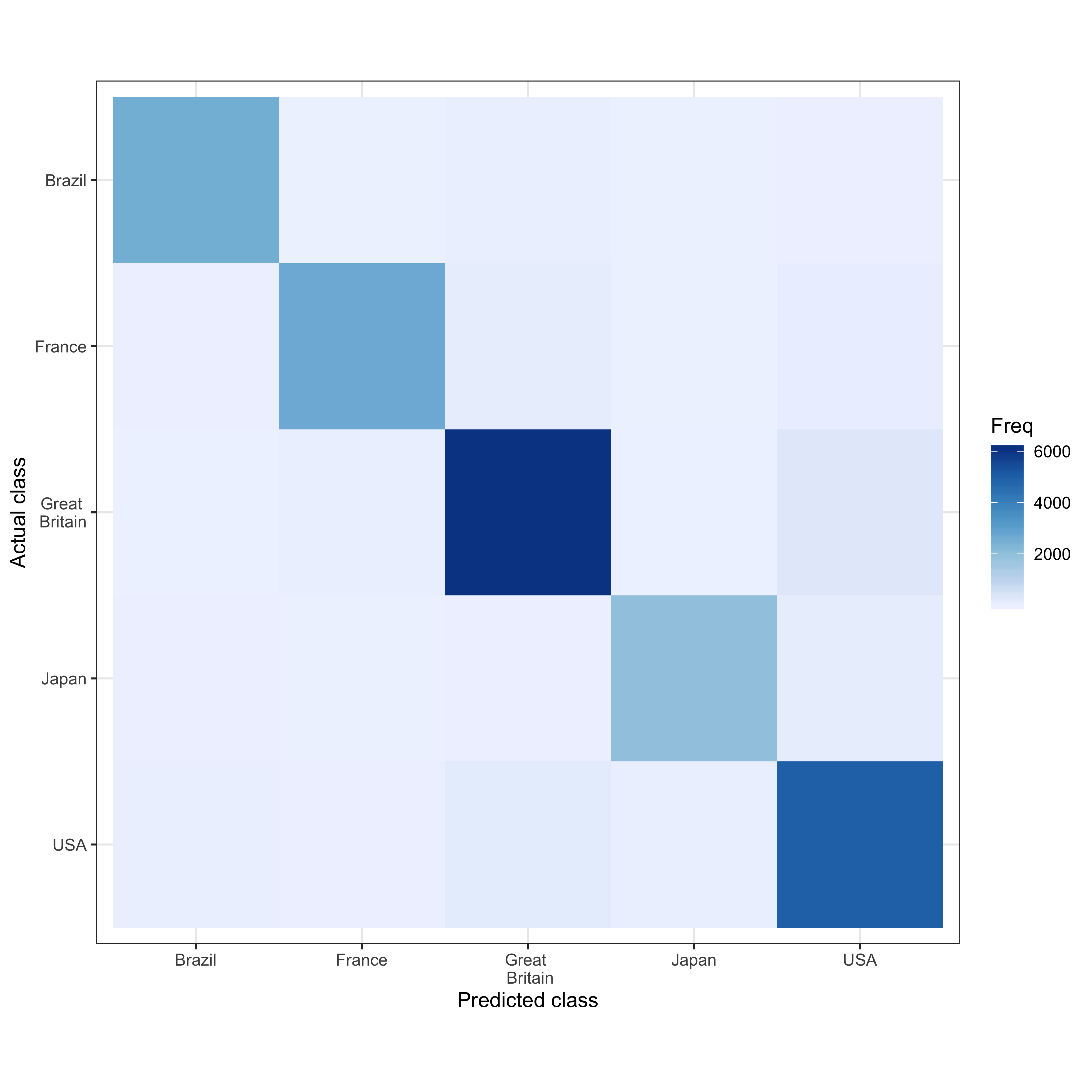
Figure 4: Contingency table
To plot the following confusion matrix, we need to slightly adjust the code from this post on data visualization by Richard Traunmüller.
Code: Confusion matrix
# Generate a data matrix from the confusion table
dat <- data.matrix(confusion$table)

# Change order of column names
order.columns <- c(5, 4, 3, 2, 1)
dat <- dat[order.columns,]

par(mgp = c(1.5, .3, 0))

# Plot
plot(
  0,
  0,
  # Type of plotting symbol
  pch = "",
  # Range of x-axis
  xlim = c(0.5, 5.5),
  # Range of y-axis
  ylim = c(0.5, 6.5),
  # Suppresses both x and y axes
  axes = FALSE,
  # Label of x-axis
  xlab = "Predicted class",
  # Label of y-axis
  ylab = "Actual class",
)

# Write a for-loop that adds the bubbles to the plot
for (i in 1:dim(dat)[1]) {
  symbols(
    c(1:dim(dat)[2]),
    rep(i, dim(dat)[2]),
    circle = sqrt(dat[i,] / 9000 / pi),
    add = TRUE,
    inches = FALSE,
    fg = brewer.pal(sqrt(dat[i,] / 9000 / pi), "Blues"),
    bg = brewer.pal(sqrt(dat[i,] / 9000 / pi), "Blues")
  )
}

axis(
  1,
  col = "white",
  col.axis = "black",
  at = c(1:5),
  label = colnames(dat)
)
axis(
  2,
  at = c(1:5),
  label = rownames(dat),
  las = 1,
  col.axis = "black",
  col = "white"
)

# Add numbers to plot
for (i in 1:5) {
  text(c(1:5), rep(i, 5), dat[i,], cex = 0.8)
}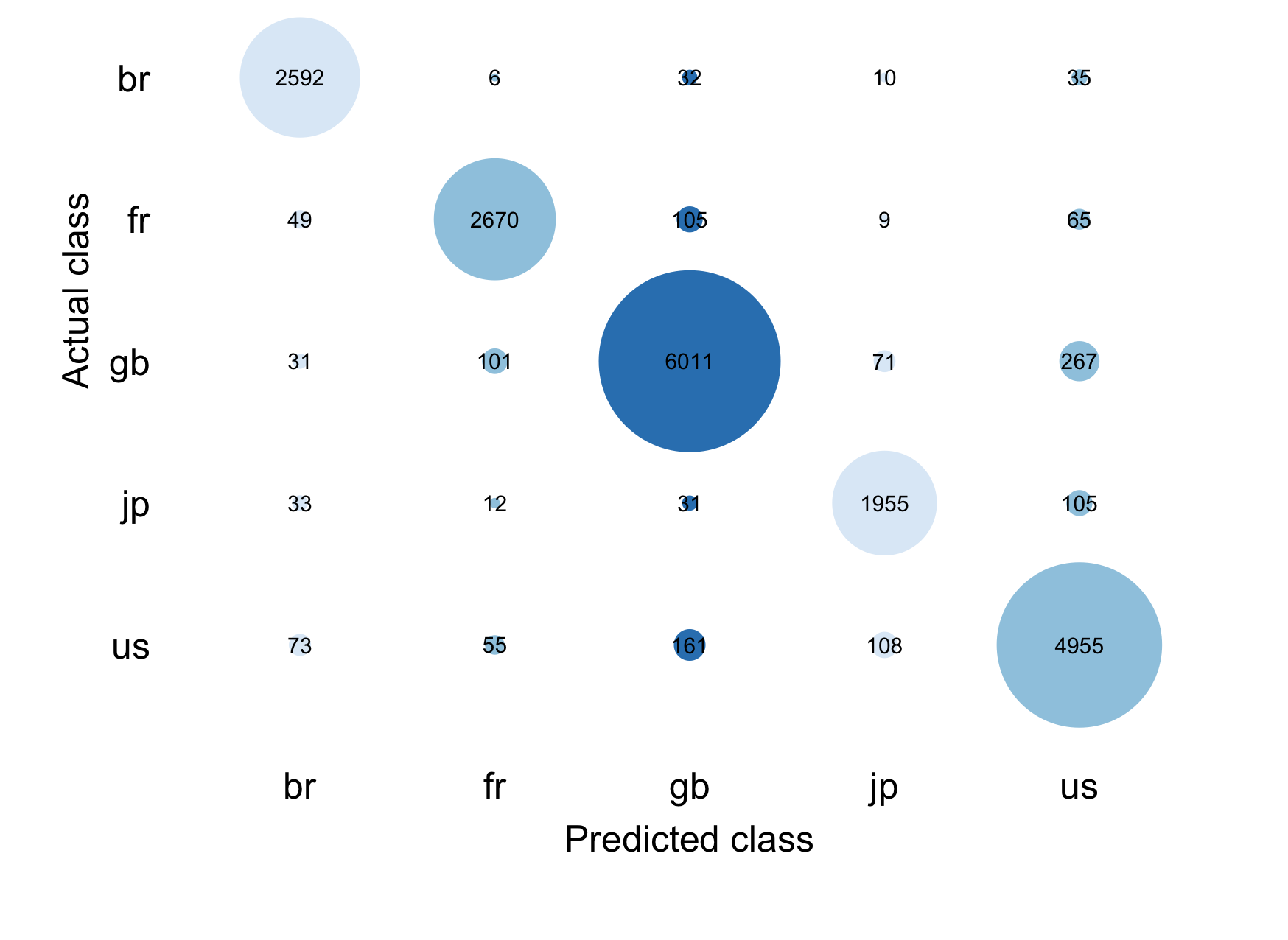
Figure 5: Contingency table
Both figures show us that our prediction performs well for all countries but it performs particularly well for the USA and Great Britain. Darker colors show a higher frequency in both plots, the contingency table also indicates a greater frequency with the size of the bubbles.
Unknown categories
Unknown categories: Unsupervised machine learning - Latent semantic analysis (LSA)
The next section addresses how to analyze texts with unknown categories. Latent Semantic Analysis (LSA) evaluates documents and seeks to find the underlying meaning or concept of these documents. If each word only had one meaning, LSA would have an easy job. However, oftentimes, words are ambiguous, have multiple meanings or are synonyms. One example from our corpus is “may” - it could be a verb, a noun for a month, or a name. To overcome this problem, LSA essentially compares how often words appear together in one document and then compares this across all other documents. By grouping words with other words, we try to identify those words that are semantically related and eventually also get the true meaning of ambiguous words. More technically, LSA is a useful technique for aligning feature distributions to an n-dimensional space. This is achieved via singular value decomposition (SVD). This decomposition allows us to decompose both a quadratic and a rectangular matrix. LSA can (among other things) be used to compare similarity of documents/documents grouped by some variable.
What are the major assumptions and simplifications that LSA has?
- Documents are non-positional (“bag of words”). The “bag of words” approach assumes that the order of the words does not matter. What matters is only the frequency of the single words.
- Concepts are understood as patterns of words where certain words often go together in similar documents.
- Words only have one meaning given the contexts surrounding the patterns of words.
For the next example, we go back to the UN General Assembly speech data set.
corpus.un.sample <- corpus_sample(mycorpus, size = 500)We again follow the cleaning steps described above.
Code: Data pre-processing steps
# Create tokens
token_sample <-
  tokens(
    split_hyphens = TRUE,
    corpus.un.sample,
    remove_numbers = TRUE,
    remove_punct = TRUE,
    remove_symbols = TRUE,
    remove_url = TRUE,
    include_docvars = TRUE
  )

# Clean tokens created by OCR
token_ungd_sample <- tokens_select(
  token_sample,
  c("[\\d-]", "[[:punct:]]", "^.{1,2}$"),
  selection = "remove",
  valuetype = "regex",
  verbose = TRUE
)

dfmat <- dfm(token_ungd_sample,
             tolower = TRUE,
             stem = TRUE,
             remove = stopwords("english")
             )
In an earlier version of this post, the function textmodel_lsa was already implemented in quanteda. It is now part of the package quanteda.textmodels. After loading the package, we can run the textmodel_lsa command.
# Load the package
library(quanteda.textmodels)

# Run the textmodel_lsa command
mylsa <- quanteda.textmodels::textmodel_lsa(dfmat, nd = 10)
One interesting question would be: How similar are the USA and Russia? Each dot represents a country-year observation. The USA are colored blue, Russia is colored red, and all other countries are grey.
# We need the "stringr" package for the following command
sources <-
  str_remove_all(rownames(mylsa$docs), "[0-9///'._txt]")

sources.color <- rep("gray", times = length(sources))
sources.color[sources %in% "USA"] <- "blue"
sources.color[sources %in% "RUS"] <- "red"

plot(
  mylsa$docs[, 4:5],
  col = alpha(sources.color, 0.3),
  pch = 19,
  xlab = "Dimension 4",
  ylab = "Dimension 5",
  main = "LSA dimensions by subcorpus"
)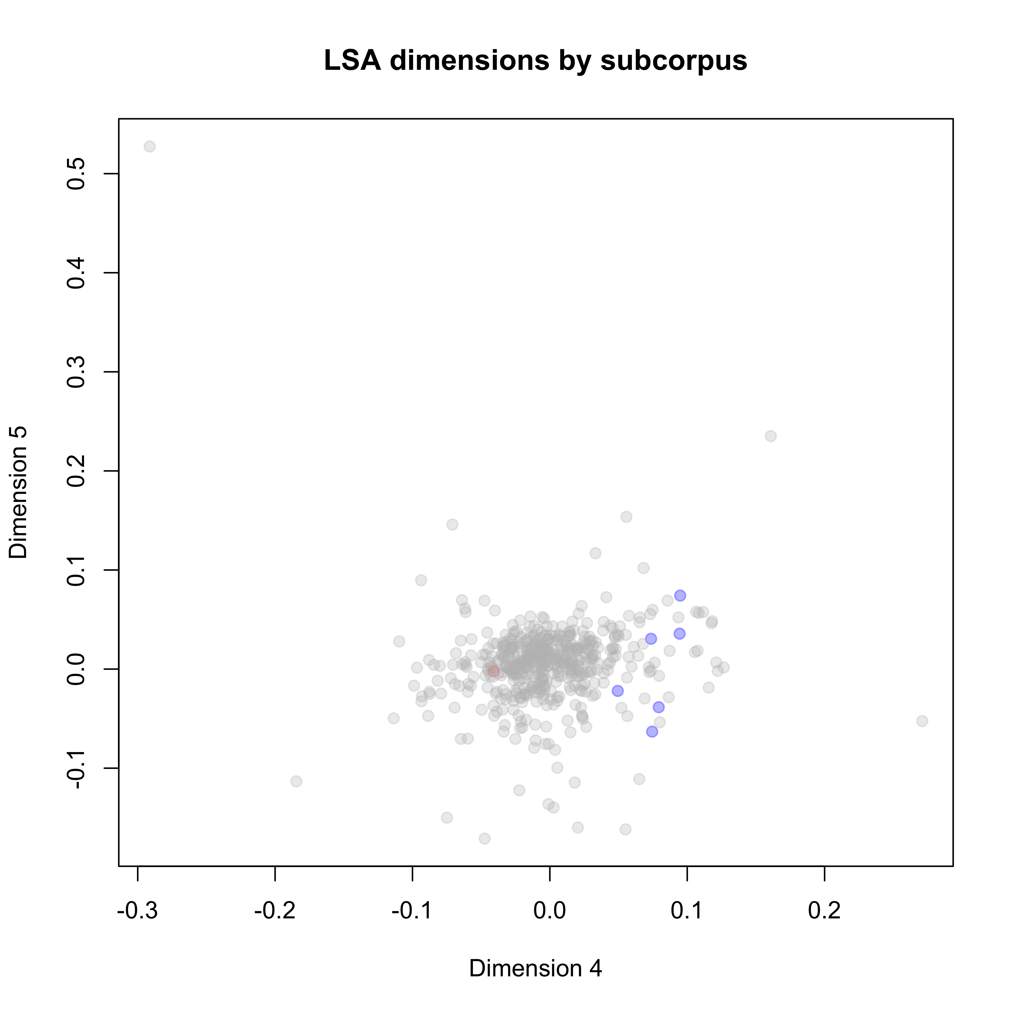
Figure 6: Distribution of PA topics in the UN General Debate corpus
On Dimension 5 we do not really observe a difference between documents from the US and Russia while we do see a topical divide on Dimension 4.
# create an LSA space; return its truncated representation in the low-rank space
tmod <- quanteda.textmodels::textmodel_lsa(dfmat[1:10, ])
# matrix in low_rank LSA space
tmod$matrix_low_rank[, 1:5] forti third session general assembl
GNQ_43_1988.txt 4.000000e+00 6.000000e+00 10 12 9
UZB_64_2009.txt -6.306067e-14 -1.748601e-15 2 1 1
PRT_50_1995.txt 2.000000e+00 -2.962543e-13 5 8 4
VCT_70_2015.txt -4.979003e-14 -1.879096e-13 3 1 6
GUY_67_2012.txt -7.959952e-14 -1.302430e-14 3 6 2
MDG_34_1979.txt -1.627830e-13 7.000000e+00 14 13 6
CHL_60_2005.txt -1.064461e-13 2.000000e+00 5 3 4
GTM_68_2013.txt -1.319652e-13 5.002986e-14 6 7 11
GIN_64_2009.txt -1.256287e-13 1.000000e+00 5 5 2
LBN_59_2004.txt -9.672818e-14 1.000000e+00 2 4 5We now fold the queries into the space generated by dfmat[1:10,] and return its truncated versions of its representation in the new low-rank space. For more information on this, see Deerwester et al. (1990) and Rosario (2000).
pred <- predict(tmod, newdata = dfmat[1:10, ])
pred$docs_newspace
10 x 10 Matrix of class "dgeMatrix"
[,1] [,2] [,3] [,4] [,5] [,6]
GNQ_43_1988.txt -0.3587033 0.04626331 -0.40268736 0.75368464 -0.198343099 0.15890426
UZB_64_2009.txt -0.1304653 0.04983523 -0.06010142 -0.07259054 0.057245087 -0.03112114
PRT_50_1995.txt -0.5120486 0.45389699 0.69697128 0.03247785 -0.071841805 0.18464906
VCT_70_2015.txt -0.2241820 0.09965473 -0.36666157 -0.45680821 -0.462552853 0.28818827
GUY_67_2012.txt -0.2905706 0.05927260 -0.29307648 -0.35382563 0.366086659 0.47269539
MDG_34_1979.txt -0.4919563 -0.83849245 0.20130813 -0.06146108 -0.038858129 -0.05927530
CHL_60_2005.txt -0.2663441 0.20190586 -0.13824724 -0.23099427 -0.006964881 -0.67210030
GTM_68_2013.txt -0.2074862 0.05127196 -0.13858784 -0.11930716 0.021618854 -0.33022555
GIN_64_2009.txt -0.2738299 0.12184387 -0.19025526 0.13644592 0.659835350 -0.13044787
LBN_59_2004.txt -0.1625876 0.12082658 -0.11439537 0.04220718 -0.408458883 -0.22780319
[,7] [,8] [,9] [,10]
GNQ_43_1988.txt 0.13239767 0.10535490 0.203828010 -0.065029344
UZB_64_2009.txt -0.21573385 -0.08282906 -0.130474714 -0.947070625
PRT_50_1995.txt 0.07183401 0.00858728 -0.005558773 0.020944555
VCT_70_2015.txt 0.35837271 -0.38370263 -0.152115117 0.029859727
GUY_67_2012.txt -0.34813601 0.38234056 0.254633069 0.106243837
MDG_34_1979.txt -0.01837620 -0.06738449 0.012211891 0.023580112
CHL_60_2005.txt 0.04450401 -0.07554420 0.596888043 0.009695998
GTM_68_2013.txt 0.35028911 0.66063039 -0.502174774 -0.007009133
GIN_64_2009.txt 0.03757466 -0.49043679 -0.361551806 0.174062011
LBN_59_2004.txt -0.74478679 -0.03668237 -0.337785293 0.234975826Unknown categories: Unsupervised machine learning - Latent Dirichlet Allocation (LDA)
Both Latent Dirichlet Allocation (LDA) and Structural Topic Modeling (STM) belong to topic modelling. Topic models find patterns of words that appear together and group them into topics. The researcher decides on the number of topics and the algorithms then discover the main topics of the texts without prior information, training sets or human annotations.
LDA is a Bayesian mixture model for discrete data where topics are assumed to be uncorrelated. It is a model that describes how the documents in a dataset were created. We assign an arbitrary number of topics (K) where each topic is a distribution over a fixed vocabulary. Each document is considered as a collection of words, one for each of K topics. It also follows the “bag of words” approach that considers each word in a document separately.
To calculate the LDA models, we need to load the package topicmodels. If you use this package for the first time on your machine, you need to execute a specific sequence of commands, detailed in the code below.
Code: Installing the package
topicmodels
# 1) Install GSL
# We first need to make sure that GSL (e.g. 'brew install gsl' in the terminal) is installed on our machine

# 2) Install gsl
# Then we proceed and choose either of the following commands:
# A)
install.packages("gsl")
# or B)
install.packages(
  "https://cran.rstudio.com/src/contrib/gsl_2.1-6.tar.gz",
  repos = NULL,
  method = "libcurl"
)

# 3) Load the gsl package
library(gsl)

# 4) Install topicmodels
# Here we choose again either of the following commands:
# A)
install.packages("topicmodels")
# or B)
install.packages(
  "https://cran.r-project.org/src/contrib/topicmodels_0.2-8.tar.gz",
  repos = NULL,
  method = "libcurl"
)

# 5) Load the topicmodels package
library(topicmodels)

# Now you are all set for the following models.
For the LDA, we again first trim our DFM. As above, the command dfm_trim trimms the text. This allows us to filter words that appear less than 7.5% and more than 90%.
mydfm.un.trim <-
  dfm_trim(
    mydfm,
    min_docfreq = 0.075,
    # min 7.5%
    max_docfreq = 0.90,
    # max 90%
    docfreq_type = "prop"
  )
We then assign an arbitrary topic number and convert the trimmed DFM to a topicmodels object.
# Assign an arbitrary number of topics
topic.count <- 15

# Convert the trimmed DFM to a topicmodels object
dfm2topicmodels <- convert(mydfm.un.trim, to = "topicmodels")
Eventually, we can calculate the LDA model with quanteda’s LDA() command.
lda.model <- LDA(dfm2topicmodels, topic.count)Output for
lda.model
lda.modelA LDA_VEM topic model with 15 topics.as.data.frame(terms(lda.model, 6))| topic1 | topic2 | topic3 | topic4 | topic5 | topic6 | topic7 | topic8 | topic9 | topic10 |
|---|---|---|---|---|---|---|---|---|---|
| nuclear | cooper | problem | trade | america | arab | arab | global | oper | war |
| weapon | council | interest | problem | american | small | palestinian | cooper | negoti | today |
| republ | reform | hope | product | latin | nuclear | israel | social | conflict | now |
| soviet | global | possibl | per | respect | issu | territori | order | problem | power |
| relat | effect | now | economi | law | pacif | isra | futur | confer | live |
| disarma | process | even | increas | principl | weapon | resolut | common | south | mani |
| topic11 | topic12 | topic13 | topic14 | topic15 |
|---|---|---|---|---|
| global | terror | african | deleg | africa |
| sustain | council | africa | session | south |
| climat | terrorist | republ | problem | independ |
| chang | iraq | conflict | concern | african |
| challeng | resolut | democrat | great | namibia |
| goal | law | elect | republ | struggl |
How similar are the fifteen topics? This question is particularly interesting because it allows us to (possibly) cluster homogeneous topics. To get a better idea of our LDA model and about the similarity among the different topics, we can plot our results using the following chunck of code. dist and hclust are standard R commands that allow us to calculate the similarity.
lda.similarity <- as.data.frame(lda.model@beta) %>%
  scale() %>%
  dist(method = "euclidean") %>%
  hclust(method = "ward.D2")

par(mar = c(0, 4, 4, 2))
plot(lda.similarity,
     main = "LDA topic similarity by features",
     xlab = "",
     sub = "")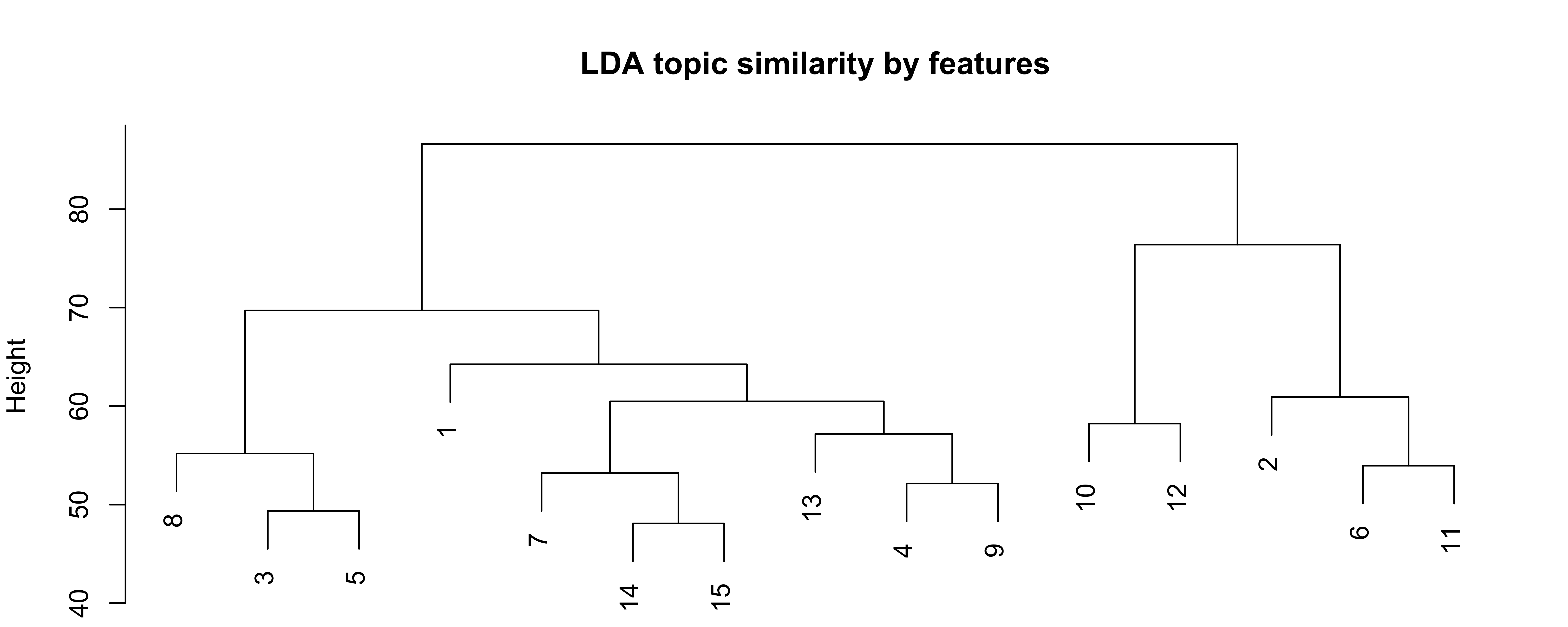
Figure 7: LDA topic similarity by features
The plot is called dendogram and visualizes a hierarchial clustering. The x-axis gives you the topics and the clusters of these topics. Put differently, it gives you information on the smilarity of the topics. On the y-axis, we see the dissmilarity (or distance) between our fifteen topics.
Unknown categories: Unsupervised machine learning - Structural topic models (STM)
The structural topic models (STM) are a popular extension of the standard LDA models. The STM allows to include metadata (the information about each document) into the topicmodel and it offers an alternative initialization mechanism (“Spectral”). For STMs, the covariates can be used in priors. The stm vignette provides a good overview how to use a STM. The package includes estimation algorithms and tools for every stage of the workflow. A particularly large emphasis is on a number of diagnostic functions that are integrated into the R package.
The package stiminsights is very useful for visual exploration. It allows the user to process interactive validation, interpretation and visualization of one or several Structural Topic Models (stm).
We again trim our dfm with the command dfm_trim.
mydfm.un.trim <-
  dfm_trim(
    mydfm,
    min_docfreq = 0.075,
    # min 7.5%
    max_docfreq = 0.90,
    # max 90%
    docfreq_type = "prop"
  )
We then assign the number of topics arbitrarily.
topic.count <- 25 # Assigns the number of topicsAnd eventually convert the DFM (with convert()) and calculate the STM (with stm()).
# Calculate the STM
dfm2stm <- convert(mydfm.un.trim, to = "stm")

model.stm <- stm(
  dfm2stm$documents,
  dfm2stm$vocab,
  K = topic.count,
  data = dfm2stm$meta,
  init.type = "Spectral"
)
To get a first insight, we print the terms that appear in each topic.
as.data.frame(t(labelTopics(model.stm, n = 10)$prob))| V1 | V2 | V3 | V4 | V5 | V6 | V7 | V8 | V9 |
|---|---|---|---|---|---|---|---|---|
| council | lebanon | soviet | global | african | nuclear | european | trade | african |
| reform | arab | union | sustain | africa | weapon | europ | economi | situat |
| effect | resolut | relat | challeng | republ | treati | cooper | product | guinea |
| activ | problem | militari | chang | democrat | disarma | union | industri | africa |
| cooper | territori | forc | climat | millennium | arm | conflict | resourc | particular |
| strengthen | palestinian | republ | goal | commit | test | process | increas | hope |
| convent | withdraw | arm | commit | poverti | non | stabil | market | concern |
| role | principl | war | agenda | particular | prolifer | contribut | price | solut |
| confer | solut | socialist | respons | like | pakistan | bosnia | global | session |
| contribut | war | polici | address | summit | india | respect | financi | problem |
| V10 | V11 | V12 | V13 | V14 | V15 | V16 | V17 | V18 |
|---|---|---|---|---|---|---|---|---|
| council | problem | cooper | republ | power | africa | order | problem | israel |
| iraq | now | stabil | korea | great | south | principl | session | arab |
| resolut | oper | dialogu | democrat | viet | debt | social | oper | palestinian |
| law | negoti | terror | china | deleg | deleg | univers | confer | isra |
| aggress | hope | sudan | south | coloni | hope | cultur | solut | palestin |
| charter | agreement | call | korean | territori | process | today | resolut | east |
| violat | mani | process | asia | nam | environ | life | cyprus | middl |
| iraqi | last | promot | north | republ | confer | respect | concern | resolut |
| islam | way | commit | east | sea | welcom | societi | negoti | occupi |
| iran | possibl | issu | cooper | charter | conflict | becom | disarma | territori |
| V19 | V20 | V21 | V22 | V23 | V24 | V25 |
|---|---|---|---|---|---|---|
| island | today | per | terror | america | conflict | africa |
| small | war | cent | afghanistan | american | refuge | south |
| pacif | live | social | afghan | latin | war | independ |
| caribbean | want | educ | cooper | central | somalia | african |
| chang | terror | poverti | terrorist | respect | assist | struggl |
| ocean | mani | health | problem | social | humanitarian | regim |
| issu | let | drug | global | process | mani | namibia |
| sea | now | democraci | asia | solut | elect | apartheid |
| climat | everi | programm | central | possibl | situat | coloni |
| call | know | million | issu | express | forc | racist |
The following plot allows us to intuitively get information on the share of the different topics at the overall corpus.
plot(
  model.stm,
  type = "summary",
  text.cex = 0.5,
  main = "STM topic shares",
  xlab = "Share estimation"
)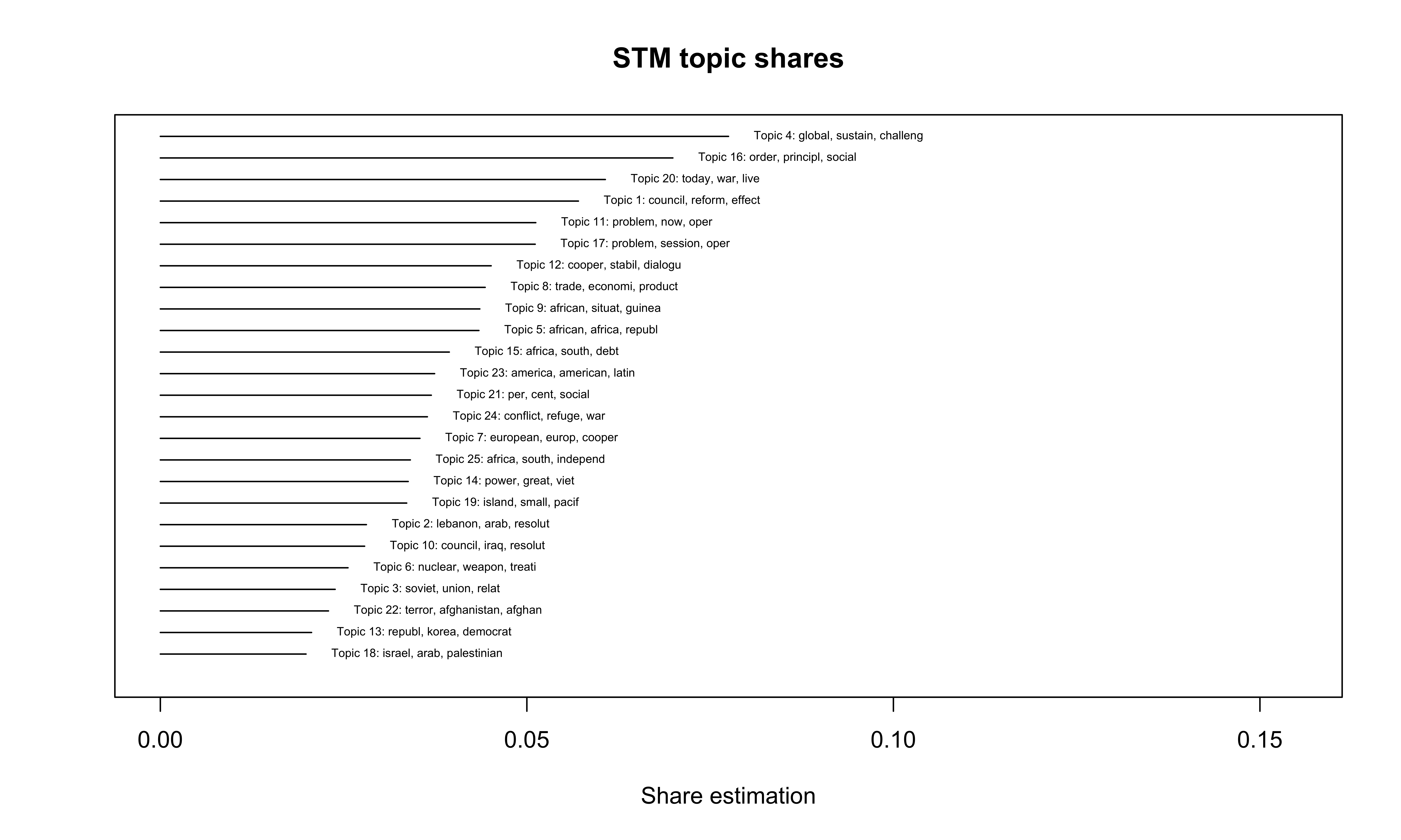
Figure 8: STM topic shares
Using the package stm, we can now visualize the different words of a topic with a wordcloud. Since topic 4 has the highest share, we use it for the next visualization. The location of the words is randomized and changes each time we plot the wordcloud while the size of the words is relative to their frequency and remains the same.
stm::cloud(model.stm,
           topic = 4,
           scale = c(2.25, .5))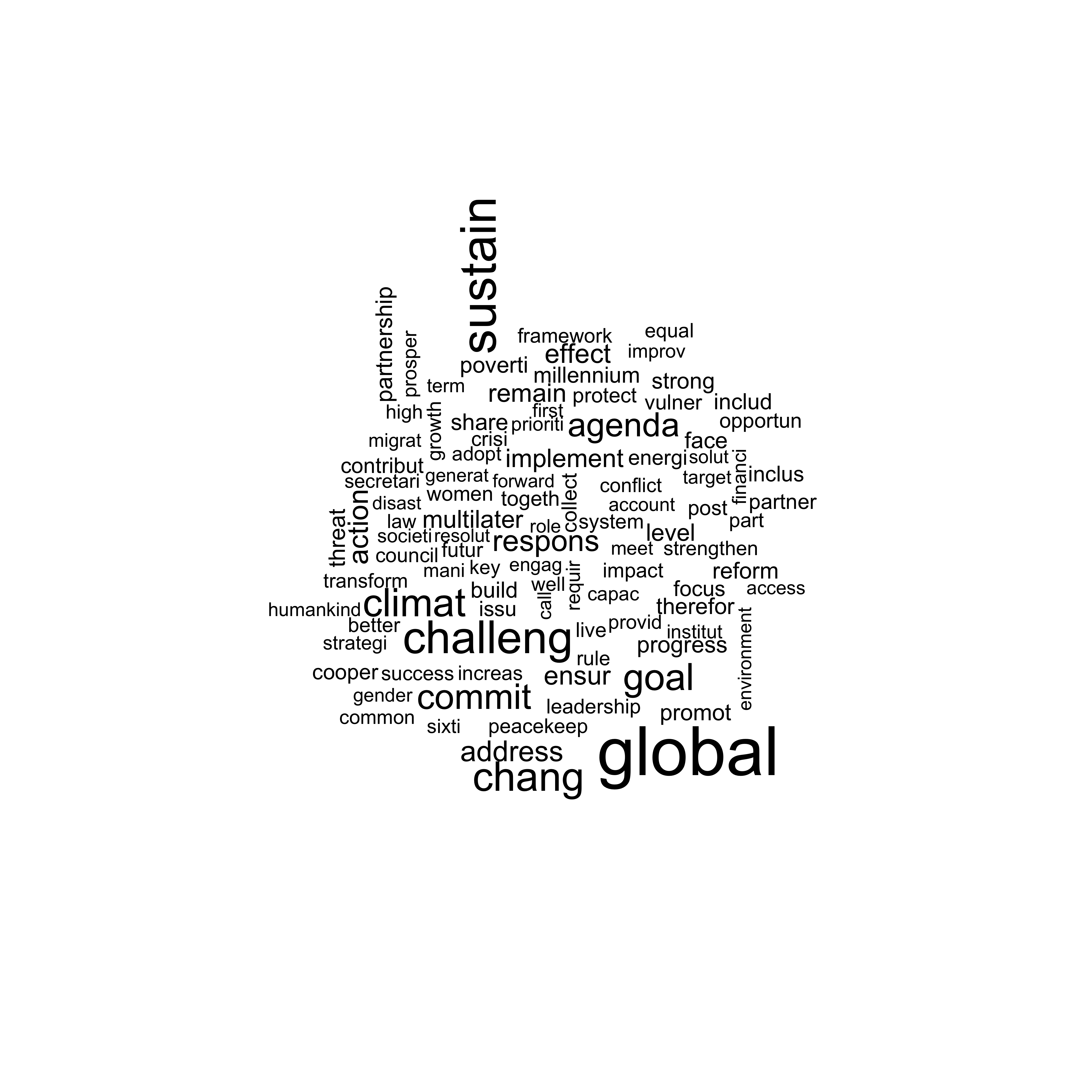
Figure 9: Wordcloud with stm
If we want, we can also put several different topics in visually perspective using the following lines of code:
plot(model.stm,
     type = "perspectives",
     topics = c(4, 5),
     main = "Putting two different topics in perspective")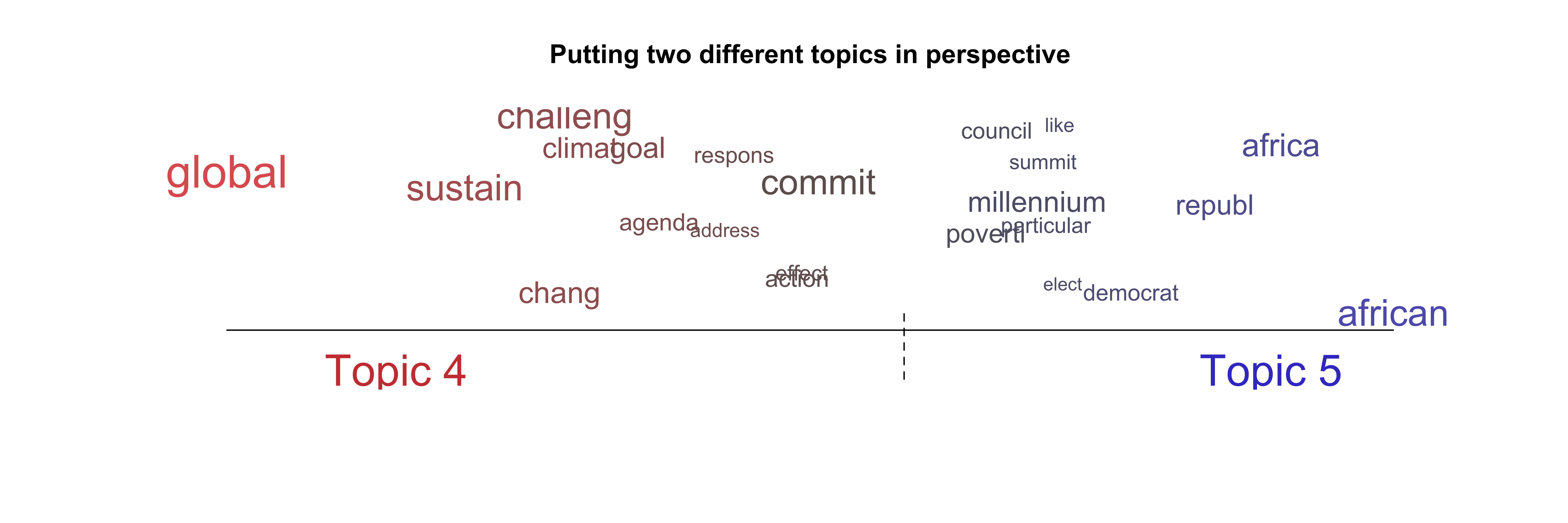
Figure 10: Wordcloud using stm – Perspective plots
The perspective plot visualizes the combination of two topics (here topic 4 and topic 5). The size of the words is again relative to their frequency (within the combination of the two topics). The x-axis shows the dregree that specific words align with Topic 4 or Topic 5. Global is closely aligned with Topic 4 whereas commit is more central in both topics.
Further readings
- quanteda: Quantitative Analysis of Textual Data
- Benoit, K., & Nulty, P.. 2016. Quanteda: Quantitative Analysis of Textual Data.
- Benoit, K., Watanabe, K., Wang, H., Nulty, P., Obeng, A., Müller, S., & Matsuo, A. (2018). quanteda: An R package for the quantitative analysis of textual data. Journal of Open Source Software, 3(30), 774.
- Deerwester, S., Dumais, S. T., Furnas, G. W., Landauer, T. K., & Harshman, R. (1990). Indexing by latent semantic analysis. Journal of the American society for information science, 41(6), 391-407. Chicago
- Grimmer, J., & Stewart, B. M. (2013). Text as data: The promise and pitfalls of automatic content analysis methods for political texts. Political Analysis, 21(3), 267-297.
- Mueller, S. Quanteda Cheat Sheet.
- Puschmann, C. Inhaltsanalyse mit R.
- Puschmann, C. Automatisierte Inhaltsanalyse mit R.
- Puschmann, C. Automatisierte Inhaltsanalyse mit R. Überwachtes maschinelles Lernen.
- Roberts, M. E., Stewart, B. M., & Tingley, D. (2014). stm: R package for structural topic models. R package, 1, 12.
- Rosario, B. (2000). Latent semantic indexing: An overview. Technical Report. INFOSYS, 240, 1-16.
- Welbers, K., Van Atteveldt, W., & Benoit, K. (2017). Text analysis in R. Communication Methods and Measures, 11(4), 245-265.
About the presenter
Cornelius Puschmann is professor of media and communication at ZeMKI, University of Bremen and an affiliate researcher at the Leibniz Institute for Media Research in Hamburg. His research interests center on online hate speech, the role of algorithms for the selection of media content, and methodological aspects of computational social science.
